
Research article · 2019 · Full text
International Journal of Statistics and Applied MathematicsForecasting Monthly Sugar Cane Yields Using Box-Jenkin’s Predictive Models in Kenya
Volume 4(6) · Pages 147–151
Research areasSugarcane Cultivation and ProcessingEnergy Load and Power Forecasting
Abstract
Author-writtenSugarcane is the main raw material in the production of sugar in Kenya. The supply of sugarcane affects directly the quantity of sugar supplied in the markets. Low supply of sugarcane leads to a decline in the amount of sugar supplied to the markets and vice versa. This creates the need of determining the quantity of sugarcane supplied by the farmers to the industries to facilitate planning. This study employed Box-Jenkins predictive models in forecasting the monthly quantity of sugarcane supplied by farmers to the industries. This study will be useful to the government and sugar industries in planning by forecasting the quantity of sugarcane expected to be supplied by farmers. Secondary data on sugarcane yields was analyzed for trend and seasonal components. Kendall’s Tau test was also conducted and it yielded a significant p-value (0.001) compared to the test level (α) = 0.05. This study detrended the data and seasonal ARIMA model was fitted to the monthly sugarcane data. SARIMA (0,1,1)(0,0,0)12 was identified from a list of SARIMA models because it had the lowest Bayesian Information Criterion (BIC). The parameter was identified and a hypothesis test, based on Ljung-Box test, was conducted to determine if the model fitted the cane data. Ljung-Box statistics = 16.577 < tabulated chi-squared value = 27.59 suggesting that SARIMA (0,1,1)(0,0,0)12 fitted the monthly sugarcane data. The R2 = 0.574 indicating that the Box Jenkins model fitted the data. SARIMA (0,1,1)(0,0,0)12 was used to conduct the monthly forecasts. It was noted that the sugarcane yields increased with time.
Summary
Source-checkedPlain-language reading of the full paper, prepared with AI and checked against the text. Each point links to the authors' own words.
Why it matters
- Sugarcane is the primary raw material for sugar production in Kenya, and its supply directly impacts the amount of sugar available in markets. View evidence ↗
- Crop shortages have caused many sugar mills to operate at less than 50% capacity, leading to increased market prices for sugar. View evidence ↗
- There is a critical need to determine the quantity of sugarcane farmers supply to industries to improve planning. View evidence ↗
The question
- The study aimed to use Box-Jenkins predictive models to forecast the monthly quantity of sugarcane supplied by farmers to industries. View evidence ↗
What they did
- The researchers analyzed secondary data on sugarcane yields to identify seasonal components and trends. View evidence ↗
- Stationarity was tested using graphical procedures and the Mann Kendall trend test. View evidence ↗
- The orders of the autoregressive (p) and moving average (q) components were determined by selecting the seasonal ARIMA model with the lowest Bayesian Information Criterion (BIC). View evidence ↗
- Ljung-Box tests were used to analyze residuals and determine if the chosen model was suitable. View evidence ↗
What they found
- The Kendall's Tau test resulted in a p-value of < 0.001, which is below the 0.05 significance level, confirming that the monthly sugarcane yield data has a trend. View evidence ↗
- After differencing, the Dickey-Fuller test showed a p-value of < 0.0001, indicating that the sugarcane yield data became stationary. View evidence ↗
- The SARIMA (0,1,1)(0,0,0)12 model was selected as the most appropriate because it had the lowest BIC of 17.164. View evidence ↗
- Forecasts generated by the model indicate that sugarcane yields are expected to increase over time. View evidence ↗
What it means
- The authors conclude that their forecasting model will be a useful tool for the government and sugar industries to plan for expected sugarcane supplies. View evidence ↗
- The authors suggest that future research should use alternative trend tests, such as Sen's slope or Cox-Stuart estimation, to verify the results. View evidence ↗
- The authors recommend comparing the current SARIMA model against the Holt-Winters seasonal additive model in future studies to see if it performs better. View evidence ↗
Visual summary
1 visualsIllustrations explain the paper; they do not show study data.
Box-Jenkins Modeling Workflow
AI-generated conceptual illustration (sugarcane plants in a Kenyan field). It explains the idea and does not show study data.
View source evidence ↗Figures & tables
From the original paper Table 2
 Table 1
 Table 3
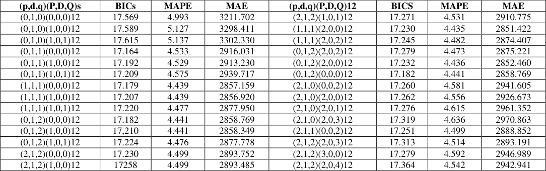 Table 4
 Table 5
 Table 6
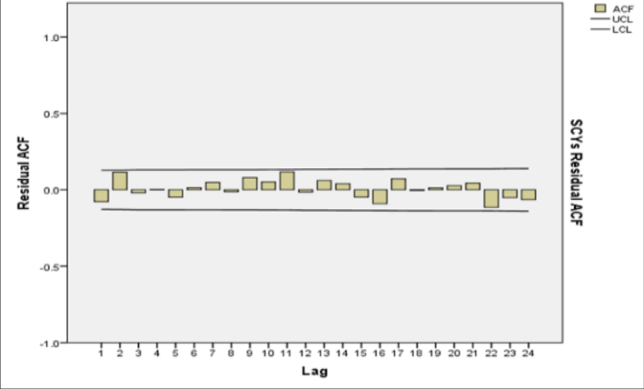 Figure 1
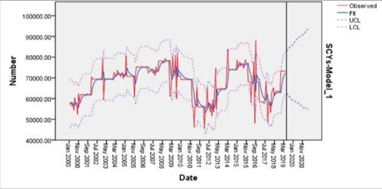 Figure 2
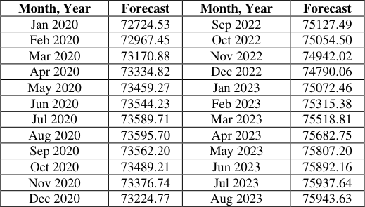 Table 7
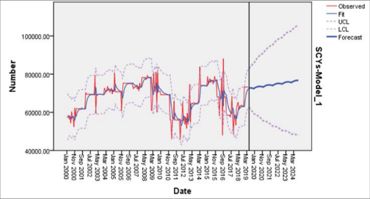 Figure 3
Introduction
Kenya's economy is dominated by the agricultural sector. Only 10% of the land area receives adequate rainfall and is able to sustain agricultural activities. Approximately 50% of the total agricultural output is meant for domestic consumption. Agricultural products are the major contributors to the country's gross domestic product (GDP). The productivity in the agricultural sector has a positive impact in the growth of the economy. To enhance growth of the Kenyan economy, it is therefore important to boost agricultural productivity (Jabuya, 2015) [1] . The quantity of sugar produced relies largely on the yields of sugarcane from farmers and the cost of production. The average cost of producing a ton of sugar in Kenya is $870 compared to $350 in Malawi and $400 in Zambia, Swaziland and Egypt and $ 450 in Sudan. The cost of production is $300 up from $270 five years ago (Bitange, 2018; Gerald, 2016) [2,3] . Though production improved from 2017, January to June in 2018 production has been declining due to cross cutting factors in the entire sugar factories. Most factories are grappling with the limited supply of sugarcane due to the crop shortage which has resulted to the mills operating below 50% of their crushing capacity. This has led to the increase of the sugar prices in the markets (Kenya News Agency, 2018) [4] . The Box-Jenkins approach to modeling ARIMA processes was described in a highly influential book by statisticians George Box and Gwilym Jenkins in 1970. According to Rob J. Hyndman, (2001) [5] : "Box-Jenkins modeling involves the identification of an appropriate ARIMA process, fitting the model to the data, and then using the fitted model for forecasting. One of the attractive features of the Box-Jenkins approach to forecasting is that ARIMA processes are a very rich class of possible models and it is usually possible to find a process which provides an adequate description to the data.
The original Box-Jenkins modeling procedure involved an iterative three-stage process of model selection, parameter estimation and model checking. The explanations of the process often add a preliminary stage of data preparation and a final stage of model application (or forecasting). This involves transformations and differencing. Transformations of the data (such as square roots or logarithms) can help stabilize the variance in a series where the variation changes with the level. This often happens with business and economic data. Then the data are differenced until there are no obvious patterns such as trend or seasonality left in the data. The "Differencing" means taking the difference between consecutive observations, or between observations a year apart. The differenced data are often easier to model than the original data. Model Selection in the Box-Jenkins framework uses various graphs based on the transformed and differenced data to try to identify potential ARIMA processes which might provide a good fit to the data. Later developments have led to other model selection tools such as Akaike's Information Criterion (AIC) and Bayesian Information Criterion (BIC). This involves finding the values of the model coefficients which provide the best fit to the data. There are sophisticated computational algorithms designed to do this. This involves testing the assumptions of the model to identify any areas where the model is inadequate. According to Rob J. Hyndman, 2001 [5] , once the model has been selected, estimated and checked, it is usually a straight forward task to compute forecasts. Of course, this is done by computer. Although originally designed for modeling time series with ARIMA processes, the underlying strategy of Box and Jenkins is applicable to a wide variety of statistical modeling situations. It provides a convenient framework which allows an analyst to think about the data, and to find an appropriate statistical model which can be used to help answer relevant questions about the data." Biljana Petrevska (2017) [6] predicted the tourism demand by Box Jenkins models in F.Y.R, Macedonia. Several alternative specifications were considered in modeling original time series. The study used the tourists recorded data for the period 1956-2013. Upon a care surgery on the ARIMA modeling procedures, the researcher identified ARIMA (1,1,1) as the most appropriate model that fits the tourism data. The model was further engaged in providing the future estimates of tourist arrivals. The study found out that there was an expectation of tourists to increase by 13.9% in 2018. ARIMA (p,d,q) model. The structure of an ARMA model is given as:
Methodology "B-J involves estimating the parameters of
Where ʎ ' s are the AR parameters, µ ' s are the MA parameters and 𝜀 are the errors
Estimation of d
This study conducted a Stationarity test to the data by using the graphical procedure and conducting a Mann Kendall trend test. The Kendall statistic is computed as:
The trend test is carried out on a time series data, 𝑌 𝑗 , that is ranked from j= 1,2,3,…,n-1 and 𝑌 𝑖 which is ranked from i= 1,2,3,…,n. Each of the data points 𝑌 𝑖 ′𝑠 is taken to be the reference points and they are compared with the other data points." That is:
According to(Robert Nyamao Nyabwanga et al, 2015): "when 𝑛 ≥ 8, the statistic k is approximately normally distributed with the mean µ and variance 𝛿 2 "This entails plotting the data over a period time and comparing the corresponding Partial autocorrelation function and/or the autocorrelation function. This study will check if the PAC and ACF do not decay to zero. This would Suggests Stationarity. If non stationary will be exhibited the data will be differenced to make it stationary. The inverse of the ACF will be checked to avoid over differencing (Florian Pelgrin, 2011) [8] . Further, this study employed the calculation of the error statistics in the chosen orders of differencing. The order with the lowest error was considered to be the best. This was done to avoid over-differencing."
Estimation of p and q
The order of p and q was estimated by comparing several a seasonal ARIMA models Bayesian Information Criterion (BIC). The model with the lowest BIC was considered to be appropriate (Florian Pelgrin, 2011) [8] . According to Box-Jenkins (1976), the MLE can be used in the estimation process of the AR and MA parameters.
Diagnostic checking
This study conducted diagnostic check by checking the Autocorrelation Plots of the residuals. This study checked if large correlation values could be identified. The correlations were determine if they were small hence determining the basis of choosing the model to conduct forecasting. Further, this study conducted the residual analyzing by employing the Ljung-Box tests as an additional step in determining the suitability of the model. Ljung-Box (S) statistics was computed as indicated here under.
Where 𝑒̂𝑘 the estimated autocorrelation of the series at lag k and L is the number of lags being tested in the analysis of the sugarcane yields data The hypothesis tested included:
H 0 : The model fits the data H A : The model does not fit the data
The hypotheses were tested at 5% significance level. In Ljung-Box test the null hypothesis is rejected when the calculated chi-squared value, at h degrees of freedom, exceeds the tabulated value. In this case h degrees of freedom are estimated such that they account for the estimated model parameters, that is ℎ = 𝐿 -𝑝 -𝑞. Where p and q are the orders of the autoregressive and moving average models (James, 2018)
Conducting P-Step Ahead Forecast
After the model had been fitted and its adequacy determined, the chosen model was used to forecast the future trend of sugarcane yields.
Results
Results
Trend Test
This study sought to determine if the data had a seasonal trend. The collected data has a seasonality of 12 months. The Kendall's trend test takes into account the seasonality of the SCYs data. The hypotheses were tested were:
H 0 : The SCYs data has no trend H A : The SCYs data has a trend
The hypothesis was tested at 5% significance level. Table 6 below shows the results of Kendall tau trend test. Since the computed P-value = < 0.001 is < significance level (α) = 0.05, we reject the null hypothesis in favor of the alternative hypothesis. Therefore, this study has established that the monthly sugarcane yields data had a trend.
| Model Fit Statistics | — | Ljung-Box | — |
|---|---|---|---|
| R2 | Statistics | df | Sig. |
| 0.574 | 16.577 | 17 | 0.483 |
Table text extracted from the original PDF; superscript letters are shown inline. The original table image is below.
View original table image
Determination of the Order of differencing
To avoid over differencing, this study ventured into the analysis of the error statistics of the different orders of differencing. The error statistics are displayed in the table below:
Model Parameters ARIMA (0,0,0)(0,1,0) is represented by A ARIMA (0,1,0)(0,0,0) is represented by B ARIMA (0,1,0)(0,1,0) is represented by C Since the computed p-value = < 0.0001 is less than the significance level = 0.05, the null hypothesis was reject and this study concluded that the differenced SCYs data was stationary.
Tentative Identification of the Model from ARIMA Class
This step involved the process of identifying the suitable seasonal ARIMA (p,d,q)(P,D,Q)s model to forecast the monthly SCYs. This study had 12 months which repeated yearly. Therefore, s = 12 in this study. This study chose the seasonal ARIMA model based on the lowest BIC. From table 4 above it can be deduced that seasonal ARIMA (0,1,1)(0,0,0)12 has the lowest BIC and hence was considered to be the most appropriate model. Seasonal ARIMA (0,1,1)(0,0,0)12 has MAPE = 4.533 and MAE = 2916.031.
| (p,d,q)(P,D,Q)s | BICs | MAPE | MAE | (p,d,q)(P,D,Q)12 | BICS | MAPE | MAE |
|---|---|---|---|---|---|---|---|
| (0,1,0)(0,0,0)12 | 17.569 | 4.993 | 3211.702 | (2,1,2)(1,0,1)12 | 17.271 | 4.531 | 2910.775 |
| (0,1,0)(1,0,0)12 | 17.589 | 5.127 | 3298.411 | (1,1,1)(2,0,0)12 | 17.230 | 4.435 | 2851.422 |
| (0,1,0)(1,0,1)12 | 17.615 | 5.137 | 3302.330 | (1,1,1)(2,0,2)12 | 17.245 | 4.482 | 2874.407 |
| (0,1,1)(0,0,0)12 | 17.164 | 4.533 | 2916.031 | (0,1,2)(2,0,2)12 | 17.279 | 4.473 | 2875.221 |
| (0,1,1)(1,0,0)12 | 17.192 | 4.529 | 2913.230 | (0,1,2)(2,0,0)12 | 17.232 | 4.436 | 2852.460 |
| (0,1,1)(1,0,1)12 | 17.209 | 4.575 | 2939.717 | (0,1,2)(0,0,0)12 | 17.182 | 4.441 | 2858.769 |
| (1,1,1)(0,0,0)12 | 17.179 | 4.439 | 2857.159 | (2,1,0)(0,0,2)12 | 17.260 | 4.581 | 2941.605 |
| (1,1,1)(1,0,0)12 | 17.207 | 4.439 | 2856.920 | (2,1,0)(2,0,0)12 | 17.262 | 4.556 | 2926.673 |
| (1,1,1)(1,0,1)12 | 17.220 | 4.477 | 2877.950 | (2,1,0)(2,0,1)12 | 17.276 | 4.615 | 2961.352 |
| (0,1,2)(0,0,0)12 | 17.182 | 4.441 | 2858.769 | (2,1,0)(2,0,3)12 | 17.319 | 4.636 | 2970.863 |
| (0,1,2)(1,0,0)12 | 17,210 | 4.441 | 2858.349 | (2,1,1)(0,0,2)12 | 17.251 | 4.499 | 2888.852 |
| (0,1,2)(1,0,1)12 | 17.224 | 4.476 | 2877.778 | (2,1,2)(2,0,3)12 | 17.313 | 4.514 | 2893.191 |
| (2,1,2)(0,0,0)12 | 17.230 | 4.499 | 2893.752 | (2,1,2)(3,0,0)12 | 17.279 | 4.592 | 2946.989 |
| (2,1,2)(1,0,0)12 | 17258 | 4.499 | 2893.485 | (2,1,2)(2,0,4)12 | 17.364 | 4.542 | 2942.941 |
Table text extracted from the original PDF; superscript letters are shown inline. The original table image is below.
View original table image
Estimation of Parameters in the Identified Model
This stage involves the estimation of the parameters and the standard errors of the identified seasonal ARIMA (0,1,1)(0,0,0)12. The series took a difference of order 1. The AR, SAR and SMA were not included in the model hence not indicated in the table 11 above. The order of the MA was 1 and the identified parameter was 0.664. The estimated standard error is 0.05. The SARIMA (0,1,1)(0,0,0)12 model took the following structure.
Where µ represents the average of the SCYs
Diagnostic Check of the Identified Model
After the tentative identification of the B-J model and computation of the parameters of the model, diagnostic check was conducted to ascertain that the model actually fits the data. This study conducted the diagnostic check by inspecting the sample ACF of the 𝑒̂𝑡.
Conclusions
Kendall Tau test of trend was also conducted. The p-value = < 0.001 is less than the significance level (α) = 0.05. This formed the basis of rejecting the null hypothesis and deducing that the SCYs data had a trend. This study fitted the SARIMA (p,d,q)(P,D,Q)s model to the SCYs data. This study fitted a Box-Jenkins model. A difference of order 1 was conducted to make the data stationary. After this, Stationarity test was conducted using the Dickey-Fuller test. The p-value = < 0.001 was less than the significance level = 0.05 indicating that the data was stationary. This study went ahead and identified, tentatively, a B-J model from the ARIMA class models. Several models were compared and it was realized that SARIMA (0,1,1)(0,0,0)12 had the lowest BIC =17.164. The corresponding MAPE and MAE for the chosen model were 4.533 and 2916.031 respectively. The parameter of the chosen model was identified. It included the MA part only, which is at lag 1 we had a parameter of 0.664. Diagnostic check was conducted to determine if the chosen model actually fitted the data. Ljung-Box test was employed. It was noted that Ljung-Box statistic = 16.577 < the tabulated chi-squared value = 27.59. Therefore this study concluded that the model fitted the SCYs data. Future researchers should fit the Holt-Winters seasonal additive model to determine if the it will perform better than the Box-Jenkins SARIMA (0,1,1)(0,0,0)12 models. The methods employed in this study could also be replicated to other statistical analysis of time series data like in the analysis of tomato yields, among others.
Acknowledgement
I wish to convey my sincere thanks to all the stakeholders and colleagues who immensely contributed in this research process. Special thanks to Jomo Kenyatta University of Agriculture and Technology for availing crucial resources that helped me in the formulation of this study.
Figures and tables from the paper
| Model | RMSE | MAPE | MAE |
|---|---|---|---|
| A | 8719.845 | 10.194 | 6625.798 |
| B | 6381.423 | 4.993 | 3211.702 |
| C | 9600.868 | 8.846 | 5797.471 |
Table text extracted from the original PDF; superscript letters are shown inline. The original table image is below.
View original table image
| Parameter | Estimate |
|---|---|
| Kendall’s Tau | 0.640 |
| P-Value | < 0.001 |
| Alpha(α) | 0.05 |
Table text extracted from the original PDF; superscript letters are shown inline. The original table image is below.
View original table image
| Tau (0bserved value) | -7.182 |
|---|---|
| Tau (critical value) | -3.420 |
| p-value (one tailed) | <0.0001 |
| α | 0.05 |
Table text extracted from the original PDF; superscript letters are shown inline. The original table image is below.
View original table image
| — | Estimate | SE |
|---|---|---|
| Difference | 1 | |
| MA Lag 1 | 0.664 | 0.050 |
Table text extracted from the original PDF; superscript letters are shown inline. The original table image is below.
View original table image
| Month, Year | Forecast | Month, Year | Forecast |
|---|---|---|---|
| Jan 2020 | 72724.53 | Sep 2022 | 75127.49 |
| Feb 2020 | 72967.45 | Oct 2022 | 75054.50 |
| Mar 2020 | 73170.88 | Nov 2022 | 74942.02 |
| Apr 2020 | 73334.82 | Dec 2022 | 74790.06 |
| May 2020 | 73459.27 | Jan 2023 | 75072.46 |
| Jun 2020 | 73544.23 | Feb 2023 | 75315.38 |
| Jul 2020 | 73589.71 | Mar 2023 | 75518.81 |
| Aug 2020 | 73595.70 | Apr 2023 | 75682.75 |
| Sep 2020 | 73562.20 | May 2023 | 75807.20 |
| Oct 2020 | 73489.21 | Jun 2023 | 75892.16 |
| Nov 2020 | 73376.74 | Jul 2023 | 75937.64 |
| Dec 2020 | 73224.77 | Aug 2023 | 75943.63 |
Table text extracted from the original PDF; superscript letters are shown inline. The original table image is below.
View original table image
References
7 in the original paper- Jabuya OD. Productivity of Sugar Factories in Kenya. Nairobi: University of Nairobi, 2015.
- Bitange N. Sour facts that blight local sugar industry. Business Daily, 2018.
- Gerald A. Kenya's Population Pushes Sugar Demand to 889,000 Tonnes. Business Daily, 2016.
- Kenya News Agency. Factrories Record Improved Sugar Production, 2018. Retrieved from business today: https://businesstoday.co.ke/factories-record-improvedsugar-production/
- Rob Hyndman J. Box-Jenkins Modelling, 2001.
- Biljana Petrevska. Prediction of Tourism Demand Using Box-Jenkins Models. Journal of Economics Research. 2017; 30(1):939-950.
- Robert Nyamao Nyabwanga et al. Statistical Trend Analysis of Residential Water Demand in Kisumu City, Kenya. American Journal of Theoretical and Applied Sciences, 2015, 112-117.
Cited by 1
From OpenAlex, OpenCitations and reference lists read by Scinovex
- Functional Time Series Models for K-Step Prediction of Sugar Production: A Case Study of Eswatini, Kenya, and South Africa ↗
Willis Oduor Agwingi, Pius Nderitu Kihara, Anthony Nyutu Karanjah · Asian Journal of Probability and Statistics · 2024
Sugar, produced from cane or beet, is a vital energy source and a globally traded commodity. Most business happens in a futures exchange market where speculators, hedgers, and institutional consumers and producers, make decisions based on their understanding of the future supply and demand situation. Sugar is sometimes bought and sold before the cane or beet is planted. Hence, improving…
❝ 0PDF