
Research article · 2019 · Full text
International Journal of Statistics and Applied MathematicsEstimation Methods of the Markov Switching GARCH Models for Forecasting Exchange Rate Volatility
Volume 6(1) · Pages 117–127
Research areasMarket Dynamics and VolatilityFinancial Risk and Volatility ModelingMonetary Policy and Economic Impact
Abstract
Author-writtenThe Markov switching GARCH model offers rich dynamics to modelling financial data. Estimating this path dependence model is a challenging task because exact computation of the likelihood is impracticable in real life. This has led to so many numerical computational methods to obtain the maximum likelihood. Just as so many numerical methods have been adopted to estimate the likelihood function, others have also adopted other methods of estimation to model this path dependence model. In this research work, the method of maximum likelihood (ML) and the Bayesian method (BM) of estimation were used in estimating the parameters of the Markov-switching GARCH model for single regime, two regime and three regime and was applied to exchange rate data. It was discovered that the three regime switching GARCH model outperformed the other regime switching model for the method of ML based on their information criteria and the two regime switching performed better based on the deviance information criteria for the BM of estimation. Furthermore, the ML performed better than the BM based on their information criteria.
Summary
Source-checkedPlain-language reading of the full paper, prepared with AI and checked against the text. Each point links to the authors' own words.
Why it matters
- Volatility clustering in financial time series occurs when large price adjustments tend to group together, creating persistent periods of high or low variance. View evidence ↗
- Markov switching generalized autoregressive conditional heteroscedastic (MSGARCH) models are highly relevant for research because they can capture the dynamics of volatility changes. View evidence ↗
- Estimating MSGARCH models is difficult because the exact computation of the likelihood function is practically infeasible due to path dependence. View evidence ↗
The question
- The study aims to compare the maximum likelihood (ML) and Bayesian (BM) estimation methods for single, two, and three-regime MSGARCH models using exchange rate data. View evidence ↗
What they did
- The researchers used monthly average Bureau de change (BDC) naira-to-dollar exchange rate data from the Central Bank of Nigeria, spanning January 1990 to December 2018. View evidence ↗
- An ARCH-LM test was performed to confirm that the exchange rate data was suitable for GARCH modeling. View evidence ↗
- For the Bayesian estimation, the study employed a GJR-GARCH model utilizing a Student's t distribution. View evidence ↗
What they found
- When using the maximum likelihood (ML) method, the three-regime switching GARCH model performed better than the single and two-regime models based on information criteria. View evidence ↗
- For the Bayesian method (BM) of estimation, the two-regime switching model was the best performer according to the deviance information criteria (DIC). View evidence ↗
- The maximum likelihood method generally outperformed the Bayesian method when compared using information criteria. View evidence ↗
- In the three-regime ML model, the probability of remaining in state 3 was 0.9029, while the probability of transitioning from state 1 to state 2 was 0.7954. View evidence ↗
- The results imply that the exchange rate is more likely to remain stable than to experience a rise at any given time. View evidence ↗
What it means
- The authors conclude that the maximum likelihood method, incorporating the MCMC approach, provides a superior estimate compared to Bayesian inference. View evidence ↗
- The authors state that increasing the number of regimes in the MS-GARCH model can lead to improved results. View evidence ↗
Visual summary
2 visualsIllustrations explain the paper; charts are replotted from the paper's own table values.
Comparison of Estimation Methods and Regimes
AI-generated conceptual illustration (Currency exchange rate data represented as a fluctuating line graph). It explains the idea and does not show study data.
View source evidence ↗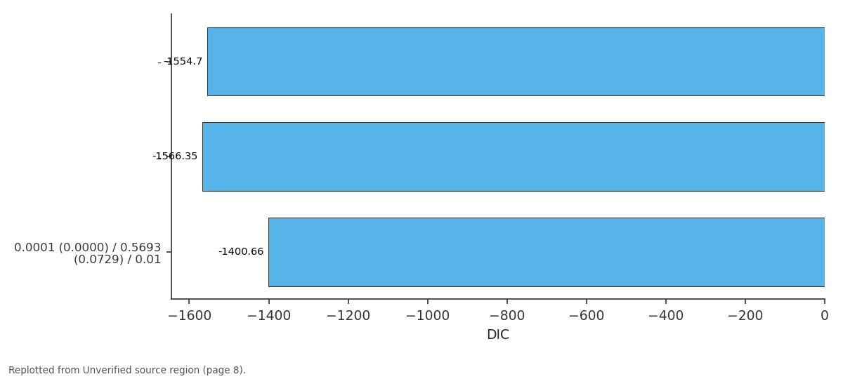
DIC: - vs - vs 0.0001 (0.0000) /...
Replotted from a table (page 8) of the original paper. Every bar is the paper's own table value.
View source evidence ↗Figures & tables
From the original paper Table 1
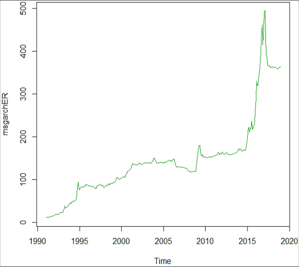 Figure 1
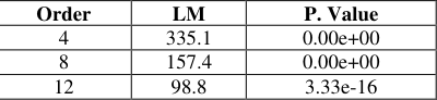 Table 2
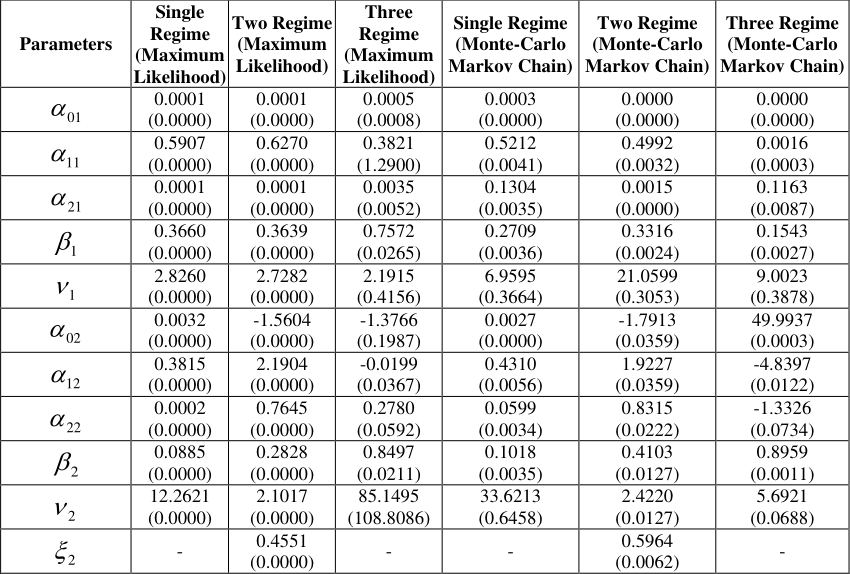 Table 3
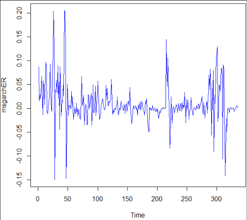 Figure 2
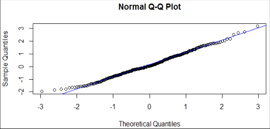 Figure 3
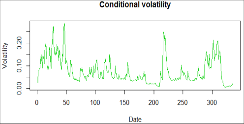 Figure 3
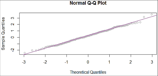 Figure 4
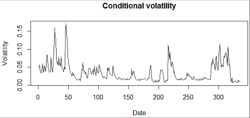 Figure 4
Introduction
In time series analysis, volatility clustering is defined as the proclivity of immense adjustments in prices of financial investments to cluster together, which results in the tenacity of these magnitudes of price changes. Mandelbrolt (1963) defined volatility clustering as “large changes tend to be followed by large changes, of either sign, and small changes tend to be followed by small changes”. If the preceding period was distinguished by high volatility, the contemporary and the imminent periods are likely to have a high variances as well. Volatility clusters are quintessential for financial price and return series, exchange rates and inflation rates.
Specifically, high frequency observations are likely to exhibit volatility clustering that can be modelled by ARCH/GARCH methods. By high frequency, we means observations that are captured monthly and below monthly observations. It is typically impervious to find ARCH/GARCH in frequencies above monthly observations (Sjo, 2011). Research on modeling volatility using time series models has burgeoned since the creation of the original ARCH model by Engle (1982) [39] and its generalization by Bollerslev (1986) [19].
From there, multiple extensions of the GARCH scedastic function have been proposed to capture additional conventionalized facts observed in financial markets, such as nonlinearities, asymmetries, and long memory properties; A review of these are seen in the work of Engle (2004). A recent work on GARCH models or GARCH models with a combination of volatility models is the novel work of Zhou et al., (2018) [76] which used the ARFIMA-IGARCH-Copula model to describe the liquidity effect in the Chinese stock market. Their result showed that the liquidity communality for the Chinese stock market was asymmetric under extreme cases. Volatility modelling generally, has found its way and has been a strong interest of research because of the various models evolving and one of these models that is of strong relevance in research is the Markov switching generalized autoregressive conditional heteroscedastic (MSGARCH) models due to the Markov Switching properties.
Maths 2021; 6(1): 117-127 Nkemnole EB Department of Mathematics, University of Lagos, Akoka, Nigeria Ebomese AP Department of Mathematics, University of Lagos, Akoka, Nigeria Nkemnole EB Department of Mathematics, University of Lagos, Akoka, Nigeria http://www.mathsjournal.com Regime Switching models, principally Markov switching (MS) models, are considered as a auspicious way to encapsulate nonlinearities in time series. They can account for variations in the structure of the mean or the variance of a process and give an uncomplicated interpretation of these shifts. Such shifts would cause regular ARMA-GARCH models to infer non-stationary processes (Henneke et al, 2007) [52]. Due to the traction of the MS and GARCH models, it is customary to combine these two approaches and consider a MS-GARCH model.
The MSGARCH model can be acknowledged as a GARCH model where parameters depend on the state of an unobserved Markov chain. One way to explain such a combination is given by Lamoureux and Lastrapes (1990) and Milkosch and Starica (2004) who conveyed that the high persistence observed in the variance of financial returns can be elucidated by time varying GARCH parameters (Augustyniak, 2013) [11]. Hamilton and Susmel (1994) [50] were among the first scholars to discuss the MS-GARCH model. They discovered that estimating this path dependent model is a challenging task because exact computation of the likelihood is infeasible in practice.
This led some authors to propose estimating modified versions of the MS-GARCH model that circumvent the path dependence problem by maximum likelihood. Gray (1996) [44], Dueker (1997) and Klaassen (2002) [60] tackle the path-dependence problem of MSGARCH through approximation, by disintegrating the past regime-specific conditional variances according to ad-hoc schemes. Other authors suggested alternative estimation methods such as a generalized method of moments (GMM) procedure which Francq and Zakoian (2008) worked on and the Bayesian Markov chain Monte Carlo (MCMC) algorithm that Bauwens et al. (2010 and 2011) worked on. Augustyniak (2013) [11] tried to answer the problem of path dependence in estimating the parameters of the MS-GARCH model.
He suggested two method of estimation, one was the Markov chain expectation maximization (MCEM) algorithm to find the maximum likelihood of the parameters of a model, and the second method was the Markov chain maximum likelihood (MCML) algorithm. He combined the two methods to form a single method called the MCEM-MCML algorithm. Ardia et al. (2017) [10] compared the method of maximum likelihood results to that of the Bayesian MCMC and did his comparison for single and two regime. We intend to extend his work to three regime switching GARCH model using exchange rate data in order to see the dynamics in this data.
A supplementary solution is to consider alternatives to traditional Maximum Likelihood estimation. Bauwens et al. (2014b) recommend to use Bayesian estimation methods that are still feasible through the so-called data augmentation techniques and particle MCMC techniques. Augustyniak (2014) depended on a Monte Carlo EM algorithm with importance sampling. In the work of Ardia (2017) [10] which we intend to extend, considered the alternative approach provided by Haas et al. (2004) [48], who let the GARCH processes of each state progress independently of the GARCH process in the other states.
Besides avoiding the path-dependence problem in traditional Maximum Likelihood estimation, their model accede for a clear cut interpretation of the variance dynamics in each regime. This model estimate is what is utilized in r programming language for the estimation of the model to be considered in this article.
Methods
Following the work of Francq et al. (2001) and the work of Bouwens et al. (2010), the MS-GARCH model can be defined by the following equations: , ) ( :1 t t t s t S y t (1) t t c t t s s t t S S S 1 :1 2 ), ( ) ( ) ( 1 :1 2 1 1 2 t t (2) . ) ( 1 1 1 1 ts t t t y S (3) Where the vector 1 2 , ,..., T y y y are the observations to be modeled and t , t=1,…,T are independently and identically distributed normal innovations with zero mean and unit variance. At each time point, the conditional mean of the observation ty is t t t t t S y y Var S where 1: 1 ty - and 1:t S are shorthand for the vectors ) | ( t t s S y E t and the conditional variance is ), , | ( ) ( :1 1 :1 :1 2 1 2 1 ( , ,..., ) t y y y - and ) , , ( 1 tS S , respectively. The process { } tS is an unobserved ergodic time homogeneous Markov chain with N-dimensional discrete state space (i.e. tS can take integer values from 1 to N). The N N transition matrix of the Markov chain N is defined by the transition probabilities j i i i i i denotes the j i t t ij i S j S p 1 , 1 ) | Pr( .
The vector ) } , , , ({ 1 , N parameters of the model. To ensure positivity of the variance, the following constraints are required: 0 ,0 i i and Augustyniak (2013) [11] in his work on maximum likelihood estimation of the Markov switching GARCH model adopted a novel approach to estimate the MS-GARCH model. One of the method he used was the Markov chain expectation maximization (MCEM) algorithm and the other was Monte Carlo Maximum likelihood algorithm. He combined the two algorithms to form a new algorithm called the new MCEM-MCML algorithm.
The combination of the two algorithms complement each other. The MCEM addresses the flaw of the MCML algorithm relating to the choice of * while the MCML method replaces many potential MCEM iterations with a single iteration, leading to a faster convergence. His method was adopted without modifications. Given an initial guess ) 0 ( the following algorithm started at 1 r = produces a sequence of iterates 1 ) ( r r allowing us to compute the MLE of the model (1-3).
To use the MCEM-MCML algorithm, the following steps are taken. 1. Simulate rm samples of the state vector S from )1 ( , | ( r y S p using a single-move Gibbs sampler. The states are simulated sequentially for T t , ,1 based on the following full conditional distribution: http://www.mathsjournal.com T (4) ) ( exp ) , , , ( ) 1 ( t T t t i y p y S S S p 2 s j j s s r i 2 1 , 1 1 t i t t :1 1 :1 2 1 t j j To ease notation, the expression 1: ( ) j t S s was reduced to j . In the context of (4), j represents ). , , ( ) 1 ( i t t i t j S S S it is 1 :1 1 ) ( straightforward to sample tS from (3.4) since tS can only take integer values from 1 to N.
However, it should be noted that it is not possible to compute expression (4) numerically for each value of tS since this will result in underflow. To avoid underflow, r m simulations we can calculate the ratios of these expressions and then recover the probabilities for 1,..., tS N = from them. The ( ) 1 { } . of the state vector S that are obtained are denoted by r i m i S = . These draws from a Markov chain with )1 ( , | ( r y S p as its stationarity distribution (Fruhwirth-Schnatter, 2006). 2.
Monte Carlo E-step: Calculate ) | (ˆ ) 1 ( r Q , an approximation of the conventional E-step ) | (ˆ ) 1 ( r Q , where r m ) ( ) 1 ( | , ( log 1 ) | (ˆ (5) i r r S y f m Q i 1 2 r r T m T m ) ( y ) 2 log( ) ( ) ( (6) s t i t r 2 ) ( s s r j t i t 1 m T 1 2 ) ( ) log( 2 2 ) ( ) log( 1 ) ( i t p m i , 1 1 i t i 1 1 i t = term 1 + term 2 3. M-step: Perform the following maximization: ). | (ˆ max arg ) 1 ( ) ( r r Q This optimization can be split into two independent steps since terms 1 and 2 of (6) involve different subsets of the parameters. Term 1 includes the mean and GARCH parameters while term 2 only contains transition probabilities. Maximization of term 1 must be performed numerically and is similar to a standard GARCH optimization to calculate the MLE.
To improve the performance of that optimization, the gradient of term 1 with respect to the mean and GARCH parameters should be provided to the optimization routine (Augustyniak, 2013) [11]. Maximization of term 2 can be done analytically. Term 2 is at its maximum when the transition probabilities take the values. f p j,k=1,…,N, jk jk N f jl i 1 r m simulated vectors. A proof of this is in Where jkf denotes the total number of transitions from state j to state k in all of the Augustyniak (2013) [11]. 4.
Apply a decision rule to determine whether to switch to MCML algorithm. If the decision is to switch, go to step 5 and set ) ( * r . Otherwise, add 1 to r and go to step 1. 5. Simulate m⋆ samples of the state vector S from ) , | ( * y S p using the single-move Gibbs sampler described in step 1 of the * ( ) algorithm to obtain the importance sample 1 { } i m i S = . 6.
MCML-step: Perform the following maximization to obtain the MLE: * m ) ( i (7) | log max arg ˆ i * 1 In contrast to the M-step, this optimization cannot be split into two step (Augustyniak, 2013) [11]. * ( ) Using importance sampling, the final sample 1 { } i m i S = , generated at step 5 of the algorithm can be transformed into a weighted http://www.mathsjournal.com ) ( * * | ) ( sample, This sample can be used to obtain an i i * ( ) ( ) * m j m | * 1 | { , } i i m i S qq v = from )ˆ , | ( y S p where . , ,1 , * ) ( i * | i 1 * m | } { ) ( j S i estimate of the smoothed inference of the state at time t, N j y S p , ,1 ), ˆ , | ( with i t I or compute the i ) ( * 1 asymptotic variance-covariance matrix of the MLE. The Bayesian estimation of the MSGARCH model was estimated. Majorly, the derivation of the student t innovation for the MSGARCH model was directly from the work of Ardia, (2009) [9]. Specifically, we used the GJR-GARCH model with the student’s t distribution.
The use of the student’s t distribution was based on the descriptive statistics carried out on the data. A Markov-switching threshold GJR (1,1) model with student-t innovations may be written as follows: 2 1) ( t t t t h e Q y for 1,..., t T = (8) iid ). ,1,0 ( ~ v S t Where } { ; ) } { } 1 { ( I K s I s I e t t t is the indicator function; the sequence tS is assumed to be a stationary, irreducible Markov process with discrete state space {1,..., } K and transition matrix [ ] ij P P = where 𝑃𝑖𝑗= ℙ(𝑠𝑡+1 = 𝑗|𝑠𝑡= 𝑖); 𝒮(0,1, 𝜐) denotes the standard Student-t density with v degrees of freedom; ( 2) / Q v v = - is the scaling factor which ensures that the conditional variance is given by t th e We define the vector of threshold GJR (1,1) conditional variance of (8) in a compact form as follows: 1 1 0 ) ( t t t t t h y y I y h (9) 1 2 1 1 2 2 Where K K K T t t h h h and . ) } { } { ( } { 1 1 1 1 ) ( ), ( ), ( , ) , , ( 1 1 1 1 K t t t y I y I y I In order to ensure the positivity of the conditional variance in every regime, we require that 0 0 and ,0 , , 2 1 , where 0 is a vector of zeros. Moreover, we require that 0 to ensure that the conditional variance is minimal when the past return is zero (i.e. when the underlying price remains constant over the last time period). Indeed, a positive threshold would yield inconsistencies such as having a return of zero affecting the volatility by more than a positive return.
It is also hard to justify why a positive return would be construed as bad news. Finally, we set 0 0 h = and 0 0 y = for convenience. The use of a Student-t instead of a Normal distribution is quite popular in standard single-regime GARCH literature. For regime- switching models, a Student-t distribution might be seen as superfluous since the switching regime can account for large unconditional kurtosis in the data.
However, as empirically observed by Klaassen (2002) [60], allowing for Student-t innovations within regimes enhances the stability of the states and allows to focus on the conditional variance’s behaviour instead of capturing some outliers. Moreover, the Student-t distribution includes the Normal distribution as the limiting case where the degrees of freedom parameter goes to infinity. We have therefore an additional flexibility in the modelling and can impose Normality by constraining the lower boundary for the degrees of freedom parameter through the prior distribution. The Student-t specification in (8) needs to be re-written in order to perform a convenient Bayesian estimation (see, e.g.
Geweke, 1993 in Ardia, 2009) [9]: 2 1) ( t t t t t h e Q y for 1,..., t T = iid ); 1,0 ( ~ N t iid . 2 , 2 ~ v v IG Where (0,1) N is a standard Normal distribution and IG the Inverted Gamma density. The degrees of freedom parameter v characterizes the density of t v as follows: v 2 v 1 1 2 (10) v v v v p 2 exp 2 2 ) | ( t t t http://www.mathsjournal.com For a parsimonious expression of the likelihood function, the vectors are defined by ) , , ( , ) , , ( , ) , , ( 1 1 1 T T T s s s y y y and ). , , , ( 3 2 1 0 The model parameters are then regrouped into ) , , ( s where ) , , , , ( P v Finally, the diagonal matrix is defined by ) } ({ ) ( 1 T t t t t h e Q diag where we recall that , t Q e and ht are both functions of the model of the parameters. Now, the likelihood function of is defined as follows: . 2 1 exp ) (det ) | ( 1 2 1 y y y L (11) This likelihood function is invariant with respect to re-labelling the states, which leads to a lack of identification of the state- specific parameters. So, without a prior inequality restriction on some state-specific parameters, a multimodal posterior is obtained and is difficult to interpret and summarize.
To overcome this problem, we make use of the permutation sampler of Fruhwirth¨- Schnatter (2001) to find suitable identification constraints. The permutation sampler requires priors that are labelling invariant. Furthermore, we cannot be completely non-informative about the state specific parameters since, from a theoretical viewpoint, this would result in improper posteriors (see, e.g. Diebolt and Robert, 1994).
In addition, a diffuse prior on τ would lead to a flat posterior since the threshold parameters are unidentified for .0 2 For the scedastic function’s parameters α, β and τ, we use truncated Normal densities I N p } 0 { ) , | ( ) ( 3 K I N p } 0 { ) , | ( ) ( K I N p } 0 { ) , | ( ) ( K Where , , and min are the hyperparameters and Nd is the d-dimensional Normal density (d>1). The assumption of labelling invariance is fulfilled if we assume that hyperparameters are the same for all states. In particular, we set min min 2 0 0 2 0 0 2 0 0 ] [, ] [, ] [, ] [, ] [, ] [, i ii i ii i ii i for 2 1 1 ] [, ] [; , ,1 ii i K i for 1,...,2 i K K = + and 2 2 2 ] [, ] [ ii i for 2 1,...,3 , i K K = + where , and min are fixed values. Note that a lower boundary min is used since the likelihood function is invariant for threshold values below the minimum value of the observed data.
Hence, the prior on could be considered to correspond to an empirical Bayes approach rather than a fully Bayesian one. The prior density of the vector conditional on v is found by noting that t are independent and identically distributed from (10), which yields: v Tv 1 T T 2 2 T v v v v p t . 2 1 exp 2 2 ) | ( (12) 1 t 1 t t Following Deschamps (2006), we choose a translated Exponential with parameters 0 and 2 for the prior on the degrees of freedom parameter: }. { )] ( exp[ ) ( v I v v p For large values of λ, the mass of the prior is concentrated in the neighbourhood of δ and a constraint on the degrees of freedom can be imposed in this manner. The Normality for the errors is obtained when δ becomes large. As pointed out by Deschamps (2006), this prior density is useful for two reasons.
First, for numerical reasons, to bound the degrees of freedom parameter away from two which avoids explosion of the conditional variance. Second, we can approximate the Normality for the errors while maintaining a reasonably tight prior that can improve the convergence of the MCMC sampler. Conditionally on the transition probability matrix P, the prior on the vector s is Markov: K K ij P s P s p N ij 1 1 1 . ) ( ) | ( i j Where 1 #{ | } ij t t N s j s i + = = = is the number of one-step transitions from state i to state j in the vector s. The mass function for the initial state, ), ( 1s is obtained by calculating the ergodic probabilities of the Markov chain (Hamilton, 1994) [50]. http://www.mathsjournal.com The prior density for the transition matrix is obtained by assuming that the K rows are independent and that the density of the ith row is dirichlet with parameter.
K K K 1 ij P D P p . ) ( ) ( i ij i 1 i 1 1 j Due to labelling invariance assumption, it is required that p ii for i=1,…,K and q ii for } ; , ,1 { , j i K j i . Finally, we form the joint prior independence between ) , (, , , and ( , ) s P . The joint posterior density is then obtained by combining the likelihood function and the joint prior via Bayes’ rule (See Ardia, 2009) [9].
Results
The data used for this analysis was gotten from the archives of the Central Bank of Nigeria (CBN). The data is a monthly data of the average Bureau de change (BDC) exchange rate of naira to dollar. The data is from January, 1990 to December, 2018. R programming language was used in the analysis of the data.
This data is archived in the repository of the Central Bank of Nigeria, 3.1 Dataset The dataset used in this article is basically the naira dollar exchange rate extracted from a pool of other exchange rates to naira. A time plot of the data is shown in figure 1. The time plot was done using R programming language. In addition, a descriptive statistics was carried out on the data.
This is seen in table 1 below. Table 1: Descriptive statistics of monthly bureau de change naira-dollar exchange rate from January, 1990 to December, 2018 Minimum Median Mean Variance Standard Deviation Maximum 10.87 137.96 146.00 8800.192 93.80934 494.70 Fig 1: Time Plot of Monthly Bureau De Change Naira-Dollar Exchange rate from January, 1990 to December, 2018 3.2 Data availability The data is available in the archives of the Central bank of Nigeria at www.cbn.gov.ng which now an open source and can be sent via email by the authors. 3.3 Data analysis Figure 1 above shows that the time plot for the data used in this article is not stationary. To confirm this, we carry out an augmented dickey fuller test which is a test for stationarity. The null hypothesis, H0, states no stationarity and the alternate hypothesis, H1, states that there is stationarity.
At 0.05 a = , the p-value for the raw data is 0.7034. The decision rule is that we fail to reject H0 and conclude that there is no enough evidence to say that the data is stationary. This implies that our raw data is not stationary. This coincides with what our time plot is actually telling us that our data is not stationary since from the time plot it does not show that it follows a white noise process.
Thus, we move to make our data stationary. To achieve this, we take the Difference of the log of the raw data. The plot is seen in figure 2 below. http://www.mathsjournal.com Fig 2: Time plot of the transformed data of monthly bureau de change naira-dollar exchange rate from January, 1990 to December, 2018 We can see from figure 2 that the plotted data seems to follow a white noise process which we can say that the data is stationary. But for us to be sure that our data is stationary, we carry out again the augmented Dickey Fuller test to see if our transformed data is stationary.
At 0.05 a = , the p-value for the test is 0.01. This implies that the data is stationary. Since in this case, the null hypothesis is rejected in favour of the alternate hypothesis. The alternate hypothesis in this case states that the data is stationary.
Thus, we fulfil the condition of stationarity which is one of the assumptions in time series modelling. An ARCH-LM test was also carried out to see if the data is suitable for the GARCH model and the result from the test shows that the data is suitable for the GARCH model. The table of results is in table 2 below. Table 2: ARCH LM test of monthly bureau de change naira-dollar exchange rate from January, 1990 to December, 2018 Order LM P.
| Order | LM | P. Value |
|---|---|---|
| 4 | 335.1 | 0.00e+00 |
| 8 | 157.4 | 0.00e+00 |
| 12 | 98.8 | 3.33e-16 |
Table text extracted from the original PDF; superscript letters are shown inline. The original table image is below.
View original table image
Value 4 335.1 0.00e+00 8 157.4 0.00e+00 12 98.8 3.33e-16 In estimating the parameters of the Markov switching GARCH models, we employed two method of estimation: the maximum likelihood method and the Monte-Carlo Markov chain method. The results for the parameters of the estimates for these two
Methods
of estimation are shown in the table 3 below. Table 3: Parameter Estimates for MSGARCH Models of Monthly Bureau De Change Naira-Dollar Exchange rate from January, 1990 to December, 2018 Two Regime Single Regime Three Regime Parameters (Maximum Likelihood) (Monte-Carlo Markov Chain) Two Regime (Monte-Carlo Markov Chain) (Monte-Carlo Markov Chain) Single Regime (Maximum Likelihood) Three Regime (Maximum Likelihood) 0.0001 (0.0000) 0.0001 (0.0000) 0.0005 (0.0008) 0.0003 (0.0000) 0.0000 (0.0000) 0.0000 (0.0000) 01 0.5907 (0.0000) 0.6270 (0.0000) 0.3821 (1.2900) 0.5212 (0.0041) 0.4992 (0.0032) 0.0016 (0.0003) 11 0.0001 (0.0000) 0.0001 (0.0000) 0.0035 (0.0052) 0.1304 (0.0035) 0.0015 (0.0000) 0.1163 (0.0087) 21 0.3660 (0.0000) 0.3639 (0.0000) 0.7572 (0.0265) 0.2709 (0.0036) 0.3316 (0.0024) 0.1543 (0.0027) 1 2.8260 (0.0000) 2.7282 (0.0000) 2.1915 (0.4156) 6.9595 (0.3664) 21.0599 (0.3053) 9.0023 (0.3878) 1 0.0032 (0.0000) -1.5604 (0.0000) -1.3766 (0.1987) 0.0027 (0.0000) -1.7913 (0.0359) 49.9937 (0.0003) 02 0.3815 (0.0000) 2.1904 (0.0000) -0.0199 (0.0367) 0.4310 (0.0056) 1.9227 (0.0359) -4.8397 (0.0122) 12 0.0002 (0.0000) 0.7645 (0.0000) 0.2780 (0.0592) 0.0599 (0.0034) 0.8315 (0.0222) -1.3326 (0.0734) 22 0.0885 (0.0000) 0.2828 (0.0000) 0.8497 (0.0211) 0.1018 (0.0035) 0.4103 (0.0127) 0.8959 (0.0011) 2 12.2621 (0.0000) 2.1017 (0.0000) 85.1495 (108.8086) 33.6213 (0.6458) 2.4220 (0.0127) 5.6921 (0.0688) 2 2 - 0.4551 (0.0000) - - 0.5964 (0.0062) - http://www.mathsjournal.com 03 - 0.0014 (0.0012) - - 0.0001 (0.0000) 13 - 0.5516 (0.4965) - - 0.5693 (0.0729) 23 - 0.0002 (0.0017) - - 0.0168 (0.0007) 3 - 0.2374 (0.3138) - - 0.3810 (0.0023) 3 - 6.6363 (3.8948) - - 3.5652 (0.0146) 11 P 0.9877 0.9906 0.0072 0.9670 0.8509 0.3710 12 P - - 0.7954 - - 0.3112 21 P 0.0441 0.0287 0.3140 0.0633 0.7682 0.2889 22 P - - 0.6860 0.0671 31 P - 0.0960 0.0088 32 P - 0.0010 0.0084 AIC -1559.0319 -1578.9851 -1591.7761 - - - BIC -1513.2623 -1529.4014 -1511.6794 - - - DIC - - -1554.7021 -1566.3519 -1400.6619 Log-Likelihood 791.5159 802.4926 816.8881 - - - Acceptance Rate - - - 27.6% 28.3% 28.4% (Standard errors) From table 3, we can see that for the method of maximum likelihood, the standard error of the estimates are all zeroes and the p- values for the method of maximum likelihood are all significant. Also, for the Bayesian inference which used the MCMC algorithm, the parameter values are the posterior mean. It is seen from table 3 that some of the standard error of the Bayesian inference were zero or close to zero.
This implies that the estimated values are close to its true population parameters. One of the reasons for this, is simply because of the simulation method used in estimating the parameters of the model. Fig 3: Volatility Forecast Plot for two Regime Switching GARCH Model (Bayesian) of Monthly Bureau De Change Naira-Dollar Exchange rate (January, 1990 to December, 2018) Figure 3 shows the conditional volatility and the QQ-plots of the residuals for two regime switching GARCH model for Bayesian estimation. From figure 3, it is seen that the QQ-plot for the residuals of the two regime switching GARCH model for Bayesian estimation follows a normal distribution.
This means that it forms a parsimonious model. In addition, the conditional volatility plots shows that it follows a Gaussian white noise process (Miller and Childers, 2012) [69]. Fig 4: Volatility Forecast Plot for three Regime Switching GARCH Model (MLE) of Monthly Bureau De Change Naira-Dollar Exchange rate from January, 1990 to December, 2018 http://www.mathsjournal.com Figure 4 shows the conditional volatility and the QQ-plots of the residuals for three regime switching GARCH model for MLE. From figure 4, it is seen that the QQ-plot for the residuals of the three regime switching GARCH model for MLE follows a normal distribution.
This means that it forms a parsimonious model. In addition, the conditional volatility plots shows that it follows a Gaussian white noise process (Miller and Childers, 2012) [69]. The transition matrix for the models revealed that the probability of remaining in one state is higher than the probability of transiting from one state to the other for both methods of estimation. For the method of maximum likelihood, the three regime switching GARCH model, the transition matrix is given by 0.0072 0.7954 0.1974 0.3140 0.6860 0.0000 0.0960 0.0010 0.9029 é ù ê ú ê ú ê ú ê ú ë û From the transition matrix above, it is seen that the probability of transiting from state 1 to state 2 is 0.7954, the probability of transiting from state 3 to state 3 that is remaining in one state is 0.9029.
This means that for the data which was used for this study, which is the exchange rate data from January 1990 to December, 2018, the probability of exchange rates to remain in the same state is 0.9029. The implication of this is that the probability for a rise in exchange rate at a particular time is relatively lower than the probability for the price of exchange rate to remain at a relatively stable price. This is also same for the Bayesian inference as the preferred model is the two regime switching GARCH model. The transition matrix is seen below. ⌊0.8250 0.1750 0.0756 0.9244⌋ Also, based on the stability of the parameters, the Bayesian inference was able to capture the shocks in the exchange rate market since some of its parameters had negative values.
Generally, in interpreting the GARCH parameters, negative values for asymmetric GARCH models implies that there were higher volatility during the period under study.
Discussion
MSGARCH models provide an explanation for the high persistence in volatility observed in single-regime GARCH models and allow for a sudden change in the (unconditional) volatility level which improves significantly the volatility forecasts (Ardia, 2009) [9]. Different parameterization of MSGARCH models have been proposed in the literature but they raise difficulties both in their estimation and their interpretation (Ardia, 2009) [9]. Haas et al. (2004) [49] overcome these problems by providing a model which can be estimated by ML and which allows for a clear-cut interpretation of the variance dynamics in each regime. In this work we employed both the method of maximum likelihood and the Bayesian inference which utilizes the Monte-Carlo Markov chain algorithm.
From the information criteria, for the method of maximum likelihood, estimation, the three regime switching GARCH model performed better than the single regime and the two regime switching GARCH models with the three regime switching GARCH model having the least akaike information criteria. Also, for the Bayesian inference, the two regime switching GARCH model performed better than single regime and the two regime switching GARCH models with the least deviance information criteria (DIC). From this article so far, we can see that the both the method of maximum likelihood and the Bayesian inference performed similarly as the differences in their information criteria weren’t so significant. The method of maximum likelihood which also employed the MCMC approach proved to be a better estimate than the Bayesian inference with an information criteria smaller than that of the Bayesian inference.
It is also noted that increasing the number of regime can also improve the result of the MS- GARCH model.
References
77 in the original paper- Albanese C, Jaimungal S, Rubisov DH. ‘A Two-state Jump Model’, Quantitative Finance 2003;3:145-154.
- Alexander C, Lazar E. On the Continuous Limit of GARCH ICMA Centre Discussion Paper in Finance 2005-13 2005a. available from www.ismacentre.rdg.ac.uk/dp
- Alexander C, Lazar E. Asymmetries and Volatility Regimes in the European Equity Markets ICMA Centre Discussion Paper in Finance 2005-14, available from www.ismacentre.rdg.ac.uk/dp
- Alexander C, Lazar E. ‘Normal Mixture GARCH (1,1): Applications to Exchange Rate Modelling’, Journal of Applied Econometrics. 2006; 21:307-336.
- Alexander C, Lazar E. Markov Switching GARCH Diffusion: ICMA Center Discussion Paper in Finance 2008-01 2008.
- Ardia D. Financial Risk Management with Bayesian Estimation of GARCH Models 2008.
- Theory and Applications, of Lecture Notes in Economics and Mathematical 612.
- Systems. Springer-Verlag, Berlin. Doi: 10.1007/978-3-540-78657-3. ISBN 978-3-540-78656-6.
- David Ardia. Bayesian estimation of a Markov‐ switching threshold asymmetric GARCH model with Student‐ t innovations. The Econometrics Journal 2009;12(1):105-126. Link: https://doi.org/10.1111/j.1368‐ 423X.2008.00253.x
- Ardia D, Bluteau K, Bout K. Forecasting performance of Markov-switching GARCH models: A large-scale empirical study Working Paper 2017.
- Augustyniak M. Maximum likelihood estimation of the Markov switching GARCH model. Computational Statistics and Data Analysis 2013. doi:10.1016/j.csda.2013.026. http://www.mathsjournal.com
- Bai X, Russell JR, Tiao GC. Beyond Merton’s Utopia (I): Effects of Non-normality and Dependence on the Precision of Variance Using High-frequency Financial Data, University of Chicago, GSB Working Paper 2001.
- Bai X, Russell JR, Tiao GC. Kurtosis of GARCH and Stochastic Volatility Models with Non-normal Innovations Journal of Econometrics 2003;114(2):349-360.
- Bakshi G, Cao C, Chen Z. Empirical Performance of Alternative Option Pricing Models, Journal of Finance 1997;52:2003- 2049.
- Barone-Adesi G, Engle R, Mancini L. GARCH Options in Incomplete Markets’, Proceedings of the ASMDA Conference 2005.
- Bauwens L, Bos CS, Van Dijk HK. Adaptive Polar Sampling with an Application to a Bayes measure of Value-at-Risk, Tinbergen Institute Discussion Paper TI 99-082/4 1999.
- Bollen NPB. Valuing Options in Regime-Switching Models, Journal of Derivatives 1998;6:38-49.
- Bollen NPB, Gray SF, Whaley RE. Regime-Switching in Foreign Exchange Rates: Evidence from Currency Option Prices, Journal of Econometrics 2000;94:239-276.
- Bollerslev T. Generalized Autoregressive Conditional heteroscedasticity, Journal of Econometrics 1986;31:309-328.
- Brown LD, Wang Y, Zhao LH. On the Statistical Equivalence at Suitable Frequencies of GARCH and Stochastic Volatility Models with Suitable Diffusion Models, University of Pennsylvania, Working paper 2002.
- Buffington J, Elliott RJ. American Options with Regime Switching, International Journal of Theoretical and Applied Finance 2002;5:497-514.
- Cai J. A Markov Model of Switching-Regime ARCH, Journal of Business and Economic Statistics 1994;12(3):309-316.
- Chourdakis K. Stochastic Volatility and Jumps Driven by Continuous Time Markov Chains, University of London Queen Mary Working Paper No. 430 2000.
- Chourdakis K. Continuous Time Regime Switching Models and Applications in Estimating Processes with Stochastic Volatility and Jumps, University of London Queen Mary Working Paper No. 464 2002.
- Chourdakis K. Non-Affine Option Pricing, Journal of Derivatives 2004;11(3):10-25.
- Corradi V. Reconsidering the Continuous Time Limit of the GARCH (1, 1) Process, Journal of Econometrics 2000;96:145- 153.
- Daal E, Yu JS. A Comparison of Mixed GARCH-Jump Models with Skewed t-Distribution for Asset Returns, SSRN Paper 2005. Available from http://ssrn.com/abstract=670502
- Di Masi GB, Kabanov YM, Runggaldier WJ. Mean-Variance Hedging of Options on Stocks with Markov Volatilities, Theory of Probability and Its Applications 1994;39:173-181.
- Ding Z, Granger CWJ. Modeling Volatility Persistence of Speculative Returns: A New Approach, Journal of Econometrics 1996;73:185-215
- Drost FC, Nijman TE. Temporal Aggregation of GARCH Processes, Econometrica 1993;61(4):909-927.
- Duan J. The GARCH Option Pricing Model, Mathematical Finance 1995;5:13-32.
- Duan J, Popova I, Ritchken P. Option Pricing under Regime Switching, Quantitative Finance 2002;2:1-17.
- Duan J, Ritchken P, Sun Z. Jump Starting GARCH: Pricing and Hedging Options with Jumps in Returns and Volatilities, Working Paper 2005a. Available from www.rotman.utoronto.ca/~jcduan/
- Duan J, Ritchken P, Sun Z. Approximating GARCH-Jump Models, Jump-Diffusion Processes, and Option Pricing, Mathematical Finance (forthcoming) 2005b.
- Duffie D, Pan J, Singleton K. Transform Analysis and Asset Pricing for Affine Jump-Diffusion, Econometrica 2000;68(6):1343-1376
- Edwards C. Derivative Pricing Models with Regime Switching: A General Approach, Journal of Derivatives Fall 2005, 41-47.
- Elliott RJ, Osakwe CJU. Option Pricing for Pure Jump Processes with Markov Switching Compensators, Finance and Stochastics 2006;10(2):250-275.
- Elliott RJ, Siu TK, Chan L. Option Pricing for GARCH Models with Markov Switching, International Journal of Theoretical and Applied Finance 2006;9(6):825-841.
- Engle RF. Autoregressive Conditional Heteroscedasticity with Estimates of the Variance of United Kingdom Inflation, Econometrica 1982;50(4):987-1007.
- Engle RF, Ng VK. Measuring and Testing the Impact of News on Volatility, Journal of Finance 1993;48:1749-1778.
- Ethier SN, Kurtz TG. Markov Processes: Characterization and Convergence, John Wiley and Sons 1986.
- Garcia R, Ghysels E, Renault E. The Econometrics of Option Pricing, forthcoming in Aït-Sahalia Y and Hansen LP (Eds.) Handbook of Financial Econometrics, Elsevier-North Holland, Amsterdam 2005.
- Glosten LR, Jagannathan R, Runkle DE. On the Relationship Between Expected Value and the Volatility of Excess Returns on Stocks, Journal of Finance 1993;48:1779-1801.
- Gray SF. Modeling the Conditional Distribution of Interest Rates as a Regime-Switching Process, Journal of Financial Economics 1996;42:27-62.
- Guo X. An Explicit Solution to an Optimal Stopping Problem with Regime Switching, Journal of Applied Probability 2001a; 38(2):464-481
- Guo X. Information and Option Pricings, Quantitative Finance 2001b;1(1):38-44.
- Guo X, Zhang Q. Closed-Form Solutions for Perpetual American Put Options with Regime Switching, SIAM Journal of Applied Mathematics 2004;64(6):2034-2049.
- Haas M, Mittnik S, Paolella MS. Mixed Normal Conditional heteroscedasticity, Journal of Financial Econometrics 2004a;2(2):211-250.
- Haas M, Mittnik S, Paolella MS. A New Approach to Markov-Switching GARCH Models, Journal of Financial Econometrics 2004b;2(4):493-530. http://www.mathsjournal.com
- Hamilton JD, Susmel R. Autoregressive Conditional Heteroscedasticity and Changes in Regime, Journal of Econometrics 1994;64:307-333.
- Hardy MR. A Regime-Switching Model of Long-Term Stock Returns’, North American Actuarial Journal 2002;5(2):41-53.
- Henneke J, Rachev S, Fabozzi F. MCMC Methods for the Estimation of MS-ARMA GARCH Models. University of California, Santa Barbera, the German Research Foundation (DFG) and the German Academic Exchange Service (DAAD) 2007.
- Heston S, Nandi S. A Closed-form GARCH Option Valuation Model, Review of Financial Studies 2000;13:585-625.
- Hwang S, Satchell SE, Valls Pereira PL. How Persistent if Volatility? An Answer with Stochastic Volatility Models with Markov Regime Switching State Equations’, Proceedings of The Econometric Society Latin American Meetings 198 2004.
- Jobert A, Rogers LCG. Option Pricing with Markov-Modulated Dynamics, SIAM Journal on Control and Optimization 2006;44(6):2063-2078.
- Johannes M. The Statistical and Economic Role of Jumps in Continuous-time Interest Rate Models, The Journal of Finance 2004;59(1):227-260.
- Jones CS. The Dynamics of Stochastic Volatility: Evidence from Underlying and Option Markets, Journal of Econometrics 2003;116:181-224.
- Jorion P. On Jump Processes in the Foreign Exchange and Stock Markets, The Review of Financial Studies 1988;1(4):427- 445.
- Kalimpalli M, Susmel R. Regime-Switching Stochastic Volatility and Short-Term Interest Rates, Journal of Empirical Finance 2004;11(3):309-329.
- Klaassen F. Improving GARCH Volatility Forecasts with Regime-Switching GARCH, Empirical Economics 2002;27:363- 394.
- Klein GE. Reply to A Regime-Switching Model of Long-Term Stock Returns by M. Hardy, April 2001, North American Actuarial Journal 2002;6(1):171-176.
- Klüppelberg C, Lindner A, Maller R. A Continuous Time GARCH Process Driven by Lévy Process 2004.
- Stationarity and Second Order Behaviour, Journal of Applied Probability 43(3):601-622.
- Konikov M, Madan DB. Option Pricing using Variance Gamma Markov Chains, Review of Derivatives Research 2002;5(1):81-115.
- Kushner HJ. Numerical Methods for Stochastic Control Problems in Continuous Time, SIAM Journal of Control and Optimization 1990;28(5):999-1048.
- Maheu JM, McCurdy TH. News Arrival, Jump Dynamics, and Volatility Components for Individual Stock Returns, The Journal of Finance 2004;59(2):755-793.
- Naik V, Lee M. General Equilibrium Pricing of Options on the Market Portfolio with Discontinuous Returns, Review of Financial Studies 1990;3:493-521.
- Nelson DB. ARCH Models as Diffusion Approximations, Journal of Econometrics 1990;45:7-38.
- Miller SL, Childers D. Probability and Random Processes (Second Edition). Elsevier Academic Press 2012.
- Siu TK, Tong H, Yang H. On Pricing Derivatives under GARCH Models: A Dynamic Gerber-Shiu Approach, North American Actuarial Journal 2004;8(3):17-31.
- Smith DR. Markov-Switching and Stochastic Volatility Diffusion Models of Short-Term Interest Rates, Journal of Business and Economic Studies 2002;20(2):183-197.
- Stroock DW, Varadhan SRS. Multidimensional Diffusion Processes, Springer-Verlag 1996.
- Timmermann A. Moment of Markov Switching Models, Journal of Econometrics 2000;96:75-111.
- Vlaar PJG, Palm FC. The Message in Weekly Exchange Rates in the European Monetary System: Journal of Business and Economic Statistics 1993;11(3):351-60. DOI: 10.1080/07350015.1993.10509963
- Wang Y. Asymptotic Nonequivalence of GARCH Models and Diffusions. The Annals of Statistics 2002;30:754-783.
- Xi-Wen Zhou, Zhen-Peng Tan, Mao-Hai Huang. Study of liquidity commonality in China's stock market, using an ARFIMA- IGARCH-COPULA model. Journal of Interdisciplinary Mathematics 2018;21(5):1351-1356. DOI: 10.1080/09720502.2018.1498306
- Yao DD, Zhang Q, Zhou XY. A Regime-Switching Model for European Options, in Yan H, Yin G, Zhang Q. Stochastic Processes, Optimization and Control Theory. Applications in Financial Engineering, Queuing Networks and Manufacturing Systems, Springer, 2006, 281-3.
Cited by 1
From OpenAlex, OpenCitations and reference lists read by Scinovex
- Forecasting Exchange Rate Volatility with Markov-Switching GARCH Model Estimation Methods ↗
E. B. Nkemnole, A.I. Taiwo, A. P. Ebomese · STEAM-H: Science, Technology, Engineering, Agriculture, Mathematics & Health · 2024
❝ 0