
Research article · 2018 · Full text
International Journal of Statistics and Applied MathematicsEvaluation of average outgoing quality (AOQ) for reliability acceptance sampling plan following log-logistic distribution
Volume 3(6) · Pages 91–97
Research areasAdvanced Statistical Process Monitoring
Abstract
Author-writtenQuality of the product plays vital role in acceptance sampling plan and the quality of the lot is determined by using average outgoing quality (AOQ) which is the expected quality of lots after the application of sampling inspection. This paper introduces the designing of Average Outgoing Quality (AOQ) and Average Outgoing Quality Limit (AOQL) for Reliability acceptance sampling plan for life test that follows Log-Logistic distribution. The procedure for designing a single sampling plan indexed through the Average Outgoing Quality (AOQ) is stated. A statistical software(R) is used to simulate the procedure developed and graph are constructed for the selection of AOQ values for a sampling plan under the Log-logistic model.
Summary
Source-checkedPlain-language reading of the full paper, prepared with AI and checked against the text. Each point links to the authors' own words.
Why it matters
- Product quality is critical in acceptance sampling, and Average Outgoing Quality (AOQ) is used to determine the expected quality of lots after sampling inspection. View evidence ↗
- Acceptance sampling provides a methodology for deciding whether to accept or reject a lot based on sample inspection results. View evidence ↗
- When acceptance sampling is applied to the lifetime of products, the procedure is specifically referred to as a life test. View evidence ↗
The question
- The study aims to design Average Outgoing Quality (AOQ) and Average Outgoing Quality Limit (AOQL) for a reliability acceptance sampling plan based on the log-logistic distribution. View evidence ↗
What they did
- The log-logistic distribution used in the plan is defined by a shape parameter (β) and a scale parameter (σ). View evidence ↗
- The R statistical software was used to simulate the developed procedure and construct graphs for selecting AOQ values. View evidence ↗
What they found
- The Average Outgoing Quality Limit (AOQL), representing the worst possible long-term AOQ for the illustrated plan, is 0.1215. View evidence ↗
- The producer's risk becomes approximately zero when the true mean life is 2.5 times or more than the required mean life. View evidence ↗
What it means
- The authors conclude that proposing AOQ and AOQL for truncated life tests using the log-logistic distribution is valuable because this distribution is a useful model for system reliability studies. View evidence ↗
Figures & tables
From the original paper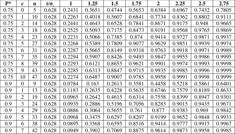 Table 1
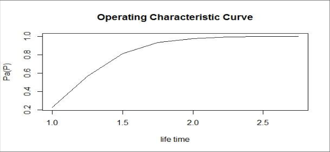 Figure 1
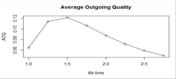 Figure 2
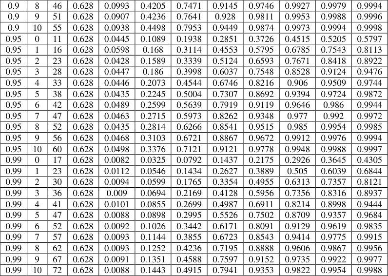 Table 2
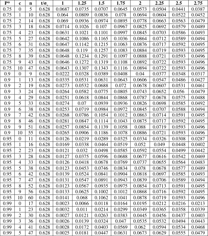 Table 2
 Table 3
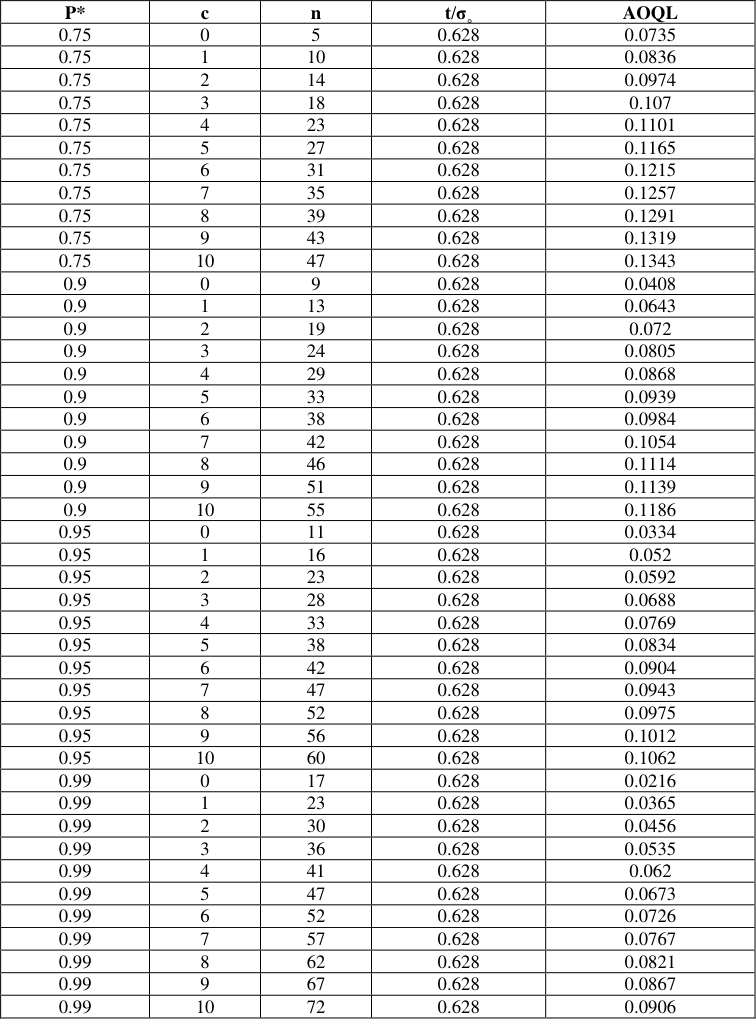 Table 3
Introduction
Acceptance sampling is one of the major areas of statistical quality control. Acceptance sampling is the methodology that deals with procedures by which decision to accept or reject the lot based on the results of the inspection of samples. Acceptance sampling prescribes a procedure that, if applied to a series of lots, will give a specified risk of accepting lots of given quality. In other words, acceptance sampling yields quality assurance and reduce the cost of inspection. The acceptance sampling could be classified in to sampling plans by attributes and sampling plans by variable. In attribute sampling plan, several sampling plans are available. For example, single sampling plan, double sampling plan and multiple sampling plan, continuous sampling plan etc. If the quality characteristic is regarding the life time of the products, then the acceptance sampling procedure is called a life test. Here it is common practice to truncate the experiment during the sampling process if no failure occurs within the experimental time period or the number of failure exceeds the specified number. Many authors have discussed acceptance sampling based on truncated life test. Epstein (1954) [1] and Sobel and Tischendrof (1959) [2] for the exponential model and The result were extended by Goode and Kao (1961) [3] for Weibull distribution, by Gupta and Groll (1961) [4] for Gamma distribution, by Kantam and Rosaiah (1998) [5] for Half Logistic distribution, by Kantam, Rosaiah and Srinivasa Rao (2001) [6] for log-logistic model, by Rosaiah, Kantam and Santosh kumar (2006) [7] for Exponentiated Log-Logistic Distribution,by Baklizi and El Masri (2004) [8] for Birnbaum-Saunders distribution, by Tsai and Wu (2006) [9] for Generalize Rayleigh distribution and by Balakrishnan et al. (2007) [10] for Generalized Birnbaum-Saunders distribution. Muhammad Hanif, Munir Ahmad and Abdur Rehman (2011) [11] developed economic reliability acceptance sampling plan from truncated life tests based on the Burr Type XII percentiles. According to ANSI / ASQC Standard A2 (1987) defines AOQ as "the expected quality" of outgoing product following the use of an acceptance sampling plan for a given value of incoming product quality and The maximum AOQ over all possible levels of incoming quality is termed as AOQL. Dodge and Romig (1959) [12] have proposed a procedure for selection of a single sampling plan (SSP) indexed through the AOQL by minimizing the average total inspection. Soundararajan (1981) [13] has suggested a procedure for the selection of an SSP in terms of the acceptable quality level (AQL) and AOQL. This paper we develop average outgoing quality and average outgoing quality limit for reliability acceptance sampling plan following log-logistic distribution when the quality characteristics follow Poisson condition. In Section 2 explains the definition of Log-Logistic distribution, Section 3 deals with the designing of the sampling plan using Log-Logistic distribution, Section 4 provides the desired operating characteristics and producer's risk, finally, Section 5 provide the average outgoing quality and average outgoing quality limit using Poisson approximation with construction of tables and numerical illustration.
Log-Logistic distribution.
Let us assume that the distribution of the life of a product is follow a Log-Logistic distribution whose cumulative distribution function ) ; (
t F
and probability density function ) ;
Where and may be called the shape and scale parameter respectively. The Log-Logistic distribution has been studied in detail by Shah & Dave (1963) [14] and Tadikamalla & Johnson (1982) [15] .
Designing of sampling plans using Log-Logistic distribution
is the failure probability and is depends only on the ratio / t
. Hence the experiment needs to specify only this ratio. The minimum values of n satisfying inequality ) 5 ( had been developed by Katam, Rosaiah and Srinivasa Rao (2001) [6] for Log-Logistic distribution.
Operating characteristic function
The operating characteristic of the sampling plan 3 ( had been developed by Kantam, Rosaiah and Srinivasa Rao (2001) [6] for Log-Logistic distribution.
Average Outgoing Quality (AOQ)
The average outgoing quality (AOQ) is the expected average quality level of the outgoing component for a given value of incoming component quality. The equation for calculation of the average outgoing quality is as follows. Step 3: For the evaluated n find 3.
N
N
Description of the Tables and Numerical Illustration
In reliability acceptance sampling plan guarantees a certain average quality as a result of the received lots. Assume that the life time distribution is a Log-Logistic distribution with 2 and that the experimenter is interested in knowing that the true unknown average lifetime is at least 1000 hours. Let the consumer's risk be set to Then the producer's risk is approximately 0.7722. The producer's risk is about zero when the true mean life is 2.5 or more times the required mean life then the producer's risk is approximately zero.
Conclusion
Quality of the product plays vital role in reliability acceptance sampling plan because in any manufacturing sector, quality is a measure or state of being free from defects (failure) So that average outgoing quality is an important measure to ensure the quality of the products. In this study, we have proposed Average outgoing Quality (AOQ) and AOQL for the truncated life test when the life time of the product follows a log-logistic distribution since the log-logistic distribution has been shown to be a useful model to analyze the system reliability studies.
Figures and tables from the paper
| P* | c | n | t/σ | 1 | 1.25 | 1.5 | 1.75 | 2 | 2.25 | 2.5 | 2.75 |
|---|---|---|---|---|---|---|---|---|---|---|---|
| 0.75 | 0 | 5 | ˳ 0.628 | 0.2431 | 0.3651 | 0.4744 | 0.5653 | 0.6384 | 0.6967 | 0.7432 | 0.7805 |
| 0.75 | 1 | 10 | 0.628 | 0.2263 | 0.4018 | 0.5607 | 0.6841 | 0.7734 | 0.8362 | 0.8802 | 0.9111 |
| 0.75 | 2 | 14 | 0.628 | 0.2441 | 0.4643 | 0.6528 | 0.7841 | 0.8671 | 0.9175 | 0.948 | 0.9665 |
| 0.75 | 3 | 18 | 0.628 | 0.2525 | 0.5093 | 0.7175 | 0.8473 | 0.9191 | 0.9568 | 0.9765 | 0.9869 |
| 0.75 | 4 | 23 | 0.628 | 0.2231 | 0.5066 | 0.7385 | 0.874 | 0.9414 | 0.9727 | 0.9871 | 0.9937 |
| 0.75 | 5 | 27 | 0.628 | 0.2268 | 0.5389 | 0.7809 | 0.9077 | 0.9629 | 0.9851 | 0.9939 | 0.9974 |
| 0.75 | 6 | 31 | 0.628 | 0.2287 | 0.5665 | 0.8149 | 0.9318 | 0.9763 | 0.9918 | 0.9971 | 0.9989 |
| 0.75 | 7 | 35 | 0.628 | 0.2294 | 0.5907 | 0.8426 | 0.9493 | 0.9847 | 0.9955 | 0.9986 | 0.9995 |
| 0.75 | 8 | 39 | 0.628 | 0.2293 | 0.6121 | 0.8655 | 0.9621 | 0.9901 | 0.9974 | 0.9993 | 0.9998 |
| 0.75 | 9 | 43 | 0.628 | 0.2285 | 0.6313 | 0.8847 | 0.9715 | 0.9935 | 0.9985 | 0.9996 | 0.9999 |
| 0.75 | 10 | 47 | 0.628 | 0.2274 | 0.6487 | 0.9007 | 0.9785 | 0.9958 | 0.9991 | 0.9998 | 0.9999 |
| 0.9 | 0 | 9 | 0.628 | 0.0784 | 0.163 | 0.2613 | 0.3581 | 0.4458 | 0.5218 | 0.5861 | 0.6401 |
| 0.9 | 1 | 13 | 0.628 | 0.1183 | 0.2635 | 0.4228 | 0.5635 | 0.6746 | 0.7579 | 0.8189 | 0.8633 |
| 0.9 | 2 | 19 | 0.628 | 0.0965 | 0.2642 | 0.4615 | 0.6314 | 0.7558 | 0.8399 | 0.8947 | 0.9301 |
| 0.9 | 3 | 24 | 0.628 | 0.0935 | 0.2886 | 0.5196 | 0.7056 | 0.8283 | 0.9015 | 0.9435 | 0.9671 |
| 0.9 | 4 | 29 | 0.628 | 0.0886 | 0.3064 | 0.5655 | 0.761 | 0.877 | 0.9383 | 0.969 | 0.9842 |
| 0.9 | 5 | 33 | 0.628 | 0.0968 | 0.3475 | 0.6297 | 0.8207 | 0.9199 | 0.9652 | 0.9848 | 0.9933 |
| 0.9 | 6 | 38 | 0.628 | 0.0895 | 0.3568 | 0.6595 | 0.8516 | 0.9414 | 0.9777 | 0.9915 | 0.9967 |
| 0.9 | 7 | 42 | 0.628 | 0.0949 | 0.3902 | 0.7069 | 0.8875 | 0.9614 | 0.9873 | 0.9958 | 0.9985 |
Table text extracted from the original PDF; superscript letters are shown inline. The original table image is below.
View original table image
| 0.9 | 8 | 46 | 0.628 | 0.0993 | 0.4205 | 0.7471 | 0.9145 | 0.9746 | 0.9927 | 0.9979 | 0.9994 |
|---|---|---|---|---|---|---|---|---|---|---|---|
| 0.9 | 9 | 51 | 0.628 | 0.0907 | 0.4236 | 0.7641 | 0.928 | 0.9811 | 0.9953 | 0.9988 | 0.9996 |
| 0.9 | 10 | 55 | 0.628 | 0.0938 | 0.4498 | 0.7953 | 0.9449 | 0.9874 | 0.9973 | 0.9994 | 0.9998 |
| 0.95 | 0 | 11 | 0.628 | 0.0445 | 0.1089 | 0.1938 | 0.2851 | 0.3726 | 0.4515 | 0.5205 | 0.5797 |
| 0.95 | 1 | 16 | 0.628 | 0.0598 | 0.168 | 0.3114 | 0.4553 | 0.5795 | 0.6785 | 0.7543 | 0.8113 |
| 0.95 | 2 | 23 | 0.628 | 0.0428 | 0.1589 | 0.3339 | 0.5124 | 0.6593 | 0.7671 | 0.8418 | 0.8922 |
| 0.95 | 3 | 28 | 0.628 | 0.0447 | 0.186 | 0.3998 | 0.6037 | 0.7548 | 0.8528 | 0.9124 | 0.9476 |
| 0.95 | 4 | 33 | 0.628 | 0.0446 | 0.2073 | 0.4544 | 0.6746 | 0.8216 | 0.906 | 0.9509 | 0.9744 |
| 0.95 | 5 | 38 | 0.628 | 0.0435 | 0.2245 | 0.5004 | 0.7307 | 0.8692 | 0.9394 | 0.9724 | 0.9872 |
| 0.95 | 6 | 42 | 0.628 | 0.0489 | 0.2599 | 0.5639 | 0.7919 | 0.9119 | 0.9646 | 0.986 | 0.9944 |
| 0.95 | 7 | 47 | 0.628 | 0.0463 | 0.2715 | 0.5973 | 0.8262 | 0.9348 | 0.977 | 0.992 | 0.9972 |
| 0.95 | 8 | 52 | 0.628 | 0.0435 | 0.2814 | 0.6266 | 0.8541 | 0.9515 | 0.985 | 0.9954 | 0.9985 |
| 0.95 | 9 | 56 | 0.628 | 0.0468 | 0.3103 | 0.6721 | 0.8867 | 0.9672 | 0.9912 | 0.9976 | 0.9994 |
| 0.95 | 10 | 60 | 0.628 | 0.0498 | 0.3376 | 0.7121 | 0.9121 | 0.9778 | 0.9948 | 0.9988 | 0.9997 |
| 0.99 | 0 | 17 | 0.628 | 0.0082 | 0.0325 | 0.0792 | 0.1437 | 0.2175 | 0.2926 | 0.3645 | 0.4305 |
| 0.99 | 1 | 23 | 0.628 | 0.0112 | 0.0546 | 0.1434 | 0.2627 | 0.3889 | 0.505 | 0.6039 | 0.6844 |
| 0.99 | 2 | 30 | 0.628 | 0.0094 | 0.0599 | 0.1765 | 0.3354 | 0.4955 | 0.6313 | 0.7357 | 0.8121 |
| 0.99 | 3 | 36 | 0.628 | 0.009 | 0.0694 | 0.2169 | 0.4128 | 0.5956 | 0.7356 | 0.8316 | 0.8937 |
| 0.99 | 4 | 41 | 0.628 | 0.0101 | 0.0855 | 0.2699 | 0.4987 | 0.6911 | 0.8214 | 0.8998 | 0.9444 |
| 0.99 | 5 | 47 | 0.628 | 0.0088 | 0.0898 | 0.2995 | 0.5526 | 0.7502 | 0.8709 | 0.9357 | 0.9684 |
| 0.99 | 6 | 52 | 0.628 | 0.0092 | 0.1026 | 0.3442 | 0.6171 | 0.8091 | 0.9129 | 0.9619 | 0.9835 |
| 0.99 | 7 | 57 | 0.628 | 0.0093 | 0.1144 | 0.3855 | 0.6723 | 0.8543 | 0.9414 | 0.9775 | 0.9915 |
| 0.99 | 8 | 62 | 0.628 | 0.0093 | 0.1252 | 0.4236 | 0.7195 | 0.8888 | 0.9606 | 0.9867 | 0.9956 |
| 0.99 | 9 | 67 | 0.628 | 0.0091 | 0.1351 | 0.4588 | 0.7597 | 0.9152 | 0.9735 | 0.9922 | 0.9977 |
| 0.99 | 10 | 72 | 0.628 | 0.0088 | 0.1443 | 0.4915 | 0.7941 | 0.9353 | 0.9822 | 0.9954 | 0.9988 |
Table text extracted from the original PDF; superscript letters are shown inline. The original table image is below.
View original table image
| P* | c | n | t/σ | 1 | 1.25 | 1.5 | 1.75 | 2 | 2.25 | 2.5 | 2.75 |
|---|---|---|---|---|---|---|---|---|---|---|---|
| 0.75 | 0 | 5 | ˳ 0.628 | 0.0687 | 0.0735 | 0.0707 | 0.0645 | 0.0573 | 0.0504 | 0.0441 | 0.0387 |
| 0.75 | 1 | 10 | 0.628 | 0.064 | 0.0809 | 0.0836 | 0.078 | 0.0694 | 0.0604 | 0.0522 | 0.0452 |
| 0.75 | 2 | 14 | 0.628 | 0.069 | 0.0936 | 0.0974 | 0.0895 | 0.0778 | 0.0663 | 0.0563 | 0.0479 |
| 0.75 | 3 | 18 | 0.628 | 0.0714 | 0.1026 | 0.107 | 0.0967 | 0.0825 | 0.0692 | 0.0579 | 0.0489 |
| 0.75 | 4 | 23 | 0.628 | 0.0631 | 0.1021 | 0.1101 | 0.0997 | 0.0845 | 0.0703 | 0.0586 | 0.0493 |
| 0.75 | 5 | 27 | 0.628 | 0.0642 | 0.1086 | 0.1165 | 0.1036 | 0.0864 | 0.0712 | 0.0589 | 0.0494 |
| 0.75 | 6 | 31 | 0.628 | 0.0647 | 0.1142 | 0.1215 | 0.1063 | 0.0876 | 0.0717 | 0.0592 | 0.0495 |
| 0.75 | 7 | 35 | 0.628 | 0.0648 | 0.119 | 0.1257 | 0.1083 | 0.0884 | 0.0719 | 0.0593 | 0.0495 |
| 0.75 | 8 | 39 | 0.628 | 0.0648 | 0.1234 | 0.1291 | 0.1097 | 0.0888 | 0.0721 | 0.0593 | 0.0496 |
| 0.75 | 9 | 43 | 0.628 | 0.0646 | 0.1272 | 0.1319 | 0.1108 | 0.0892 | 0.0722 | 0.0593 | 0.0496 |
| 0.75 | 10 | 47 | 0.628 | 0.0643 | 0.1307 | 0.1343 | 0.1116 | 0.0894 | 0.0722 | 0.0593 | 0.0496 |
| 0.9 | 0 | 9 | 0.628 | 0.0222 | 0.0328 | 0.0389 | 0.0408 | 0.04 | 0.0377 | 0.0348 | 0.0317 |
| 0.9 | 1 | 13 | 0.628 | 0.0335 | 0.0531 | 0.0631 | 0.0643 | 0.0606 | 0.0547 | 0.0486 | 0.0427 |
| 0.9 | 2 | 19 | 0.628 | 0.0273 | 0.0532 | 0.0688 | 0.072 | 0.0678 | 0.0607 | 0.0531 | 0.0461 |
| 0.9 | 3 | 24 | 0.628 | 0.0264 | 0.0582 | 0.0775 | 0.0805 | 0.0743 | 0.0652 | 0.056 | 0.0479 |
| 0.9 | 4 | 29 | 0.628 | 0.0251 | 0.0618 | 0.0844 | 0.0868 | 0.0787 | 0.0678 | 0.0575 | 0.0488 |
| 0.9 | 5 | 33 | 0.628 | 0.0274 | 0.07 | 0.0939 | 0.0936 | 0.0826 | 0.0698 | 0.0585 | 0.0492 |
| 0.9 | 6 | 38 | 0.628 | 0.0253 | 0.0719 | 0.0984 | 0.0972 | 0.0845 | 0.0707 | 0.0588 | 0.0494 |
| 0.9 | 7 | 42 | 0.628 | 0.0268 | 0.0786 | 0.1054 | 0.1012 | 0.0863 | 0.0714 | 0.0591 | 0.0495 |
| 0.9 | 8 | 46 | 0.628 | 0.0281 | 0.0847 | 0.1114 | 0.1043 | 0.0875 | 0.0717 | 0.0592 | 0.0495 |
| 0.9 | 9 | 51 | 0.628 | 0.0257 | 0.0854 | 0.1139 | 0.1058 | 0.088 | 0.0719 | 0.0593 | 0.0496 |
| 0.9 | 10 | 55 | 0.628 | 0.0265 | 0.0906 | 0.1186 | 0.1078 | 0.0886 | 0.0721 | 0.0593 | 0.0496 |
| 0.95 | 0 | 11 | 0.628 | 0.0126 | 0.0219 | 0.0289 | 0.0325 | 0.0334 | 0.0326 | 0.0308 | 0.0287 |
| 0.95 | 1 | 16 | 0.628 | 0.0169 | 0.0338 | 0.0464 | 0.0519 | 0.052 | 0.049 | 0.0448 | 0.0402 |
| 0.95 | 2 | 23 | 0.628 | 0.0121 | 0.032 | 0.0498 | 0.0585 | 0.0592 | 0.0554 | 0.0499 | 0.0442 |
| 0.95 | 3 | 28 | 0.628 | 0.0127 | 0.0375 | 0.0596 | 0.0688 | 0.0677 | 0.0616 | 0.0542 | 0.0469 |
| 0.95 | 4 | 33 | 0.628 | 0.0126 | 0.0418 | 0.0678 | 0.0769 | 0.0737 | 0.0655 | 0.0564 | 0.0483 |
| 0.95 | 5 | 38 | 0.628 | 0.0123 | 0.0453 | 0.0746 | 0.0834 | 0.078 | 0.0678 | 0.0577 | 0.0489 |
| 0.95 | 6 | 42 | 0.628 | 0.0139 | 0.0524 | 0.0841 | 0.0904 | 0.0818 | 0.0697 | 0.0585 | 0.0493 |
| 0.95 | 7 | 47 | 0.628 | 0.0131 | 0.0547 | 0.0891 | 0.0943 | 0.0839 | 0.0706 | 0.0589 | 0.0494 |
| 0.95 | 8 | 52 | 0.628 | 0.0123 | 0.0567 | 0.0935 | 0.0975 | 0.0854 | 0.0713 | 0.0591 | 0.0495 |
| 0.95 | 9 | 56 | 0.628 | 0.0133 | 0.0625 | 0.1002 | 0.1012 | 0.0868 | 0.0716 | 0.0592 | 0.0495 |
| 0.95 | 10 | 60 | 0.628 | 0.0141 | 0.068 | 0.1062 | 0.1041 | 0.0878 | 0.0719 | 0.0593 | 0.0496 |
| 0.99 | 0 | 17 | 0.628 | 0.0023 | 0.0066 | 0.0118 | 0.0164 | 0.0195 | 0.0212 | 0.0216 | 0.0213 |
| 0.99 | 1 | 23 | 0.628 | 0.0032 | 0.011 | 0.0214 | 0.0299 | 0.0349 | 0.0365 | 0.0358 | 0.0339 |
| 0.99 | 2 | 30 | 0.628 | 0.0027 | 0.0121 | 0.0263 | 0.0383 | 0.0445 | 0.0456 | 0.0437 | 0.0403 |
| 0.99 | 3 | 36 | 0.628 | 0.0026 | 0.0139 | 0.0324 | 0.047 | 0.0535 | 0.0532 | 0.0494 | 0.0443 |
| 0.99 | 4 | 41 | 0.628 | 0.0028 | 0.0172 | 0.0403 | 0.0569 | 0.062 | 0.0594 | 0.0534 | 0.0468 |
| 0.99 | 5 | 47 | 0.628 | 0.0025 | 0.0181 | 0.0447 | 0.0631 | 0.0673 | 0.0629 | 0.0555 | 0.0479 |
Table text extracted from the original PDF; superscript letters are shown inline. The original table image is below.
View original table image
| 0.99 | 6 | 52 | 0.628 | 0.0026 | 0.0207 | 0.0513 | 0.0704 | 0.0726 | 0.0659 | 0.0571 | 0.0487 |
|---|---|---|---|---|---|---|---|---|---|---|---|
| 0.99 | 7 | 57 | 0.628 | 0.0026 | 0.0231 | 0.0575 | 0.0767 | 0.0767 | 0.068 | 0.058 | 0.0491 |
| 0.99 | 8 | 62 | 0.628 | 0.0026 | 0.0252 | 0.0632 | 0.0821 | 0.0798 | 0.0694 | 0.0586 | 0.0493 |
| 0.99 | 9 | 67 | 0.628 | 0.0026 | 0.0272 | 0.0684 | 0.0867 | 0.0821 | 0.0704 | 0.0589 | 0.0495 |
| 0.99 | 10 | 72 | 0.628 | 0.0025 | 0.0291 | 0.0733 | 0.0906 | 0.0839 | 0.0709 | 0.0591 | 0.0495 |
Table text extracted from the original PDF; superscript letters are shown inline. The original table image is below.
View original table image
| P* | c | n | t/σ | AOQL |
|---|---|---|---|---|
| 0.75 | 0 | 5 | ˳ 0.628 | 0.0735 |
| 0.75 | 1 | 10 | 0.628 | 0.0836 |
| 0.75 | 2 | 14 | 0.628 | 0.0974 |
| 0.75 | 3 | 18 | 0.628 | 0.107 |
| 0.75 | 4 | 23 | 0.628 | 0.1101 |
| 0.75 | 5 | 27 | 0.628 | 0.1165 |
| 0.75 | 6 | 31 | 0.628 | 0.1215 |
| 0.75 | 7 | 35 | 0.628 | 0.1257 |
| 0.75 | 8 | 39 | 0.628 | 0.1291 |
| 0.75 | 9 | 43 | 0.628 | 0.1319 |
| 0.75 | 10 | 47 | 0.628 | 0.1343 |
| 0.9 | 0 | 9 | 0.628 | 0.0408 |
| 0.9 | 1 | 13 | 0.628 | 0.0643 |
| 0.9 | 2 | 19 | 0.628 | 0.072 |
| 0.9 | 3 | 24 | 0.628 | 0.0805 |
| 0.9 | 4 | 29 | 0.628 | 0.0868 |
| 0.9 | 5 | 33 | 0.628 | 0.0939 |
| 0.9 | 6 | 38 | 0.628 | 0.0984 |
| 0.9 | 7 | 42 | 0.628 | 0.1054 |
| 0.9 | 8 | 46 | 0.628 | 0.1114 |
| 0.9 | 9 | 51 | 0.628 | 0.1139 |
| 0.9 | 10 | 55 | 0.628 | 0.1186 |
| 0.95 | 0 | 11 | 0.628 | 0.0334 |
| 0.95 | 1 | 16 | 0.628 | 0.052 |
| 0.95 | 2 | 23 | 0.628 | 0.0592 |
| 0.95 | 3 | 28 | 0.628 | 0.0688 |
| 0.95 | 4 | 33 | 0.628 | 0.0769 |
| 0.95 | 5 | 38 | 0.628 | 0.0834 |
| 0.95 | 6 | 42 | 0.628 | 0.0904 |
| 0.95 | 7 | 47 | 0.628 | 0.0943 |
| 0.95 | 8 | 52 | 0.628 | 0.0975 |
| 0.95 | 9 | 56 | 0.628 | 0.1012 |
| 0.95 | 10 | 60 | 0.628 | 0.1062 |
| 0.99 | 0 | 17 | 0.628 | 0.0216 |
| 0.99 | 1 | 23 | 0.628 | 0.0365 |
| 0.99 | 2 | 30 | 0.628 | 0.0456 |
| 0.99 | 3 | 36 | 0.628 | 0.0535 |
| 0.99 | 4 | 41 | 0.628 | 0.062 |
| 0.99 | 5 | 47 | 0.628 | 0.0673 |
| 0.99 | 6 | 52 | 0.628 | 0.0726 |
| 0.99 | 7 | 57 | 0.628 | 0.0767 |
| 0.99 | 8 | 62 | 0.628 | 0.0821 |
| 0.99 | 9 | 67 | 0.628 | 0.0867 |
| 0.99 | 10 | 72 | 0.628 | 0.0906 |
Table text extracted from the original PDF; superscript letters are shown inline. The original table image is below.
View original table image
References
15 in the original paper- Epstein. Trunctated Life Tests in the Exponential Case, Ann. Math. Statist, 1954; 25(3):555-564.
- Sobel M, Tischendrof J. Acceptance sampling with new life test objectives, in Proceedings of 5 th National Symposium on Reliability and Quality Control, 1959, 108-118.
- Goode HP, Kao JHK. Sampling plans based on the Weibull distribution, Proceedings of the Seventh National Symposium on Reliability and Quality Control, Philadelphia, 1961, 24-40.
- Gupta SS, Groll PA. Gamma distribution in acceptance sampling based on life test, Journal of American Statistical Association. 1961; 56:942-970.
- Kantam RRL, Rosaiah K. Half logistic distribution in acceptance sampling based on life tests, IAPQR Transactions. 1998; 23(2):117-125.
- Kantam RRL, Rosaiah K, Srinivasa Rao G. Acceptance sampling based on life test: log-logistic model, Journal of Applied Statistics. 2001; 28(1):121-128.
- Rosaih K, Kantam RRL, Santosh Kumar CH. Reliability test plan for Exponentiated log-logistic distribution, Economic Quality Control. 2006; 21(2):165-175.
- Baklizi A, El Masri AEK. Acceptance Sampling plans based on truncated life tests in the Birnbaum Saunders model, Risk Analysis, 2004; 24:453-1457, 4.
- Tsai TR, Wu SJ. Acceptance sampling based on truncated life tests for generalized Rayleigh distribution, Journal of Applied Statistics. 2006; 33(6):595-600.
- Balakrishnan N, Leiva V, Lopez J. Acceptacne Samplling plans from truncated life tests based on the generalized BrinbaumSaunders distribution, Communications in Statistics: Simulation and Computation. 2007; 36(3):643-656.
- Abdur Razzaque Mugal, Muhammad Hanif, Munir Ahmad, Abdur Rehman. Economic Reliability Acceptance Sampling Plans from Truncated Life Tests based on the Burr Type XII Percentiles, Pak. J Coommer. Soc. Sci. 2011; 5(1):166-176.
- Dodge HF, Roming HG. Samplin inspection tables, 2 nd Ed, New York, NY: Wiley, 1959.
- Soundararajan V. Single sampling attributes plan indexed by AQL & AOQL. Journal of Quality Technology. 1981; 13:195200.
- Shah BK, Dave PH. A note on log-logistic distribution. J Math. Sciences University Baroda. 1963; 12:21-22.
- Tadikamalla PR, Johnson NL. Systems of frequency curves generated by transformation of logistic variables. Biometrika. 1982; 69:461-465.