
Research article · 2017 · Full text
International Journal of Statistics and Applied MathematicsBayesian analysis of dynamic correlation -multivariate stochastic volatility (DC-MSV) model
Volume 2(6) · Pages 09–15
Research areasFinancial Risk and Volatility ModelingStock Market Forecasting Methods
Abstract
Author-writtenThe forex exchange rate is the most volatile aspect in financial studies. This study uses a bayesian approach to estimate dynamic correlation multivariate stochastic volatility, a case of the Kenya stocks. Data was obtained from the Central Bank of Kenya website depicting the daily exchange rates for a period of 12 years (2003-2015). Multivariate Stochastic Volatility (MSV) model was fitted and its residuals exhibited volatility clustering hence the use Dynamic Correlation Multivariate Stochastic Volatility (DC-MSV) was applied to address these characteristics. Using Akaike Information Criterion (AIC) and Deviance Information Criterion (DIC) found that the returns are leptokurtic and have fat tails. The study estimated posterior parameters of the model by using of Markovian chain Monte Carlo (MCMC) iterations that worked well. Empirical results suggest that the best specifications are those that allow for time-varying correlation coefficients. The dynamic correlation multivariate stochastic volatility was found ideal in estimating volatility in stock exchanges.
Summary
Source-checkedPlain-language reading of the full paper, prepared with AI and checked against the text. Each point links to the authors' own words.
Why it matters
- Foreign exchange rates are considered the most volatile element within financial studies. View evidence ↗
- Accurately estimating the covariance matrix of multiple asset returns is essential for investors to identify portfolio risks and opportunities in a timely manner. View evidence ↗
- Kenya utilizes a free-floating exchange rate system, meaning market supply and demand determine the daily value of its currency. View evidence ↗
The question
- The study aims to use a Bayesian approach to estimate dynamic correlation multivariate stochastic volatility (DC-MSV) specifically for Kenyan stocks. View evidence ↗
What they did
- The researchers used daily exchange rate data from the Central Bank of Kenya spanning 12 years, from September 1, 2003, to December 22, 2015. View evidence ↗
- The analysis involved 2,750 trading days of the Kenya Shilling's average exchange rate against the US Dollar, Japanese Yen, South African Rand, Sterling Pound, and Euro. View evidence ↗
- The model's posterior parameters were estimated using Markov Chain Monte Carlo (MCMC) iterations. View evidence ↗
- The researchers used the Akaike Information Criterion (AIC) and Deviance Information Criterion (DIC) to analyze return distributions. View evidence ↗
What they found
- Analysis using AIC and DIC revealed that the returns are leptokurtic and characterized by fat tails. View evidence ↗
- The correlation process showed high persistence, with a posterior mean for ψ of 0.98. View evidence ↗
- Positive posterior means for parameters ɸ11, ɸ22, ψ, ψ0, and σ2p, with 95% credibility intervals above zero, suggest that Kenyan shilling volatility drives volatility in the Dollar, Euro, and Yen. View evidence ↗
- The data fit the model well, as indicated by the Deviance Information Criterion (DIC) values (D- = 2756.03, pD = 2741.2, and a difference of 53.52). View evidence ↗
What it means
- The authors conclude that the most effective model specifications are those that permit time-varying correlation coefficients. View evidence ↗
- The authors state that the dynamic correlation multivariate stochastic volatility (DC-MSV) model is ideal for estimating volatility in stock exchanges. View evidence ↗
Figures & tables
From the original paper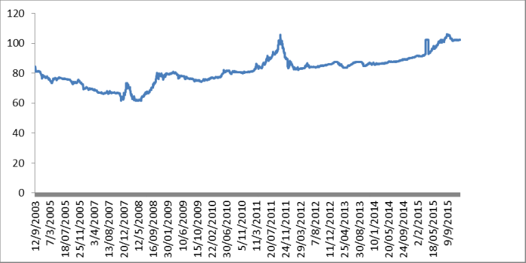 Figure 1
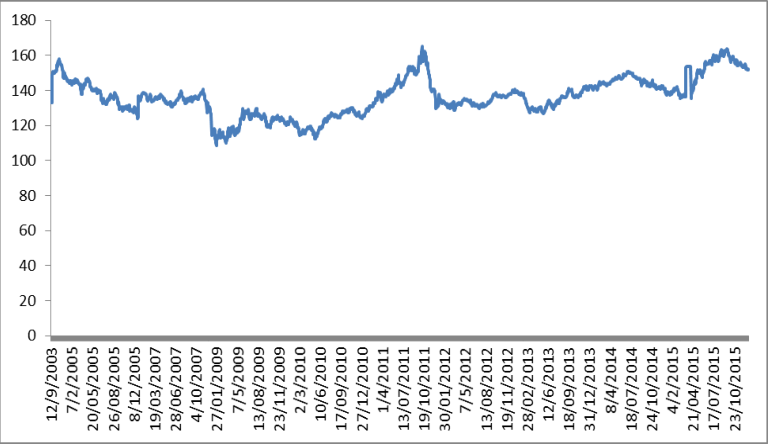 Figure 2
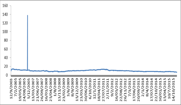 Figure 3
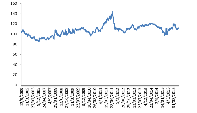 Figure 4
 Table 1
 Table 2
 Table 3
Introduction
Multivariate volatility models have proved to be a powerful inferential tool (William J.
McCausland * Universit´e de Montr´eal, CIREQ and CIRANO, 2012). They are characterized by different types of dynamic cross-sectional dependence among multiple assets returns. Research has revealed that asset return volatility varies over time, changing in response to views and revised expectations of future performance. It tends to cluster, so that large price changes tend to be followed by other large changes. Volatility is not independent across markets and assets, and this cross-sectional dependence is time-varying. Cross-sectional correlations increase substantially in periods of high market volatility, especially in bear markets. The distribution of returns is heavy tailed. There is an asymmetric relation between price and volatility changes known as the "leverage effect": increases in volatility are associated more with large decreases in price than with large increases. Multivariate volatility models that can capture these stylized facts are in high demand in finance given their many important applications, especially in modern portfolio management and exchange rate forecasting. Learning about the joint distribution of asset returns is a key element for the construction, diversification, and evaluation and hedging of portfolios. Accurate estimation of the covariance matrix of multiple asset returns allows the investor to timely identify opportunities or risks associated with a particular portfolio. It is important to track changes in Correlations to assess the risk of a portfolio, especially during periods of market stress. Financial crises usually have a strong impact on correlation. Markets tend to behave as one during big crashesas the risk of some assets increases, investors wish to sell other risky investments. The result is more highly correlated returns. The pessimistic conclusion is that diversification is least effective at reducing risk at the very times when risk is highest. An awareness of this fact avoids false optimism. Exchange rate influences, interest rate charged, inflation, imports and exports. Kenya is among many countries that embrace the free floating exchange rate system where demand and supply forces of market determine the daily value of one currency against another. The exchange rate affects the prices of directly imported goods as well as and indirectly through the local goods that are under competitive pressure from imported goods. Thus there are high rates of volatility exhibited by exchange rates. An investor with different asset returns will wish to look unto volatilities in the market before investing.
Literature Review
Volatility modeling is understood to have a constant volatility thus a poor fit of time series data while dynamic structures have provided a more realistic approach to variance modelling of returns. Several approaches have been advanced to model timevarying data. There are two main types of multivariate volatility models: observation-driven and parameter-driven. In observation-driven models, volatility is a deterministic function of observed variables, which allows straightforward evaluation of the likelihood function like multivariate GARCH type models, which are observation driven, Bauwens, Laurent, and Rombouts (2006) [4] . This study focuses on parameter-driven volatility models, also called stochastic volatility (SV) models; volatility is a latent stochastic process. Jacquier, Polson, and Rossi (1994) [14] and Geweke (1994) [10] give evidence suggesting that Stochastic Volatility (SV) models are more realistic. Stochastic processes differ with GARCH type models in terms of the structure of the model. The stochastic process depends on previous realized stocks in the series while GARCH assumes that it follows its own stochastic process with potential dependence. Bates (1996) give an overview of how to estimate the stochastic volatility models which the research will use to model the multivariate stochastic process as developed by (Harvey et al, 1994) [13] , who came up with multivariate stochastic models that later led to development of multifactor models for multivariate series (Hopes 1999, Aqillar and West 2000, and Chib Et al 2002 [1,8] . Engle (1995) [9] and Shephard (2005) [25] comprehensively reviewed the stochastic models and GARCH. Meyer and Yu (2006) [27, 28] realized that SV models are superior to GARCH type models in time series modelling. Aydemi (1998) observed that we often observe movements between markets or stocks or sectors in the exchange rates. He attributed this to a set of assets being formally linked together due to being influenced by common unobserved factors. A study by Ntawihebasenga,, Mwita, P. and Mungatu, J. (2014) on modeling volatility in exchange rate used Generalized Autoregressive Conditional Heteroscedasticity(GARCH) approach to model volatility in Rwanda Exchange rate returns. The Autoregressive (AR) model with GARCH errors was fitted to the daily exchange rate returns using Quasi-Maximum Likelihood Estimation (Q-MLE) method to get the current volatility. Asymptotic consistency and asymptotic normality of estimated parameters were given. The study showed the model fits Rwanda exchange rate returns data well. A study by Mumo, P.M. (2016) on effects of macroeconomic volatility on stock prices in Kenya. The study exploited the presence of unit roots of order 1(1) on the data set to apply the Johansen procedure and the Vector Error Correction Model (VECM) for data analysis. It was realized that both a long-run equilibrium relationship between stock prices and the macroeconomic variables and between inflation and other macro variables. The results suggested a negative long-run equilibrium relationship between money supply and stock prices. Inflation shows negative but insignificant relationship. Exchange rates and interest rates show a positive relationship. The short-term dynamics from the VECM support earlier documented evidence, implying the earlier evidence reflect short-run and not long-run dynamics. There are also more natural discrete time representations of the continuous time models upon which much of modern finance theory is based. Unfortunately, computation of the likelihood function, which amounts to integrating out latent states, is difficult. However, since the introduction of Bayesian Markov chain Monte Carlo (MCMC) methods by Jacquier, Polson, and Rossi (1994) [14] for univariate SV models, inference for these models has become much more feasible. These methods require the evaluation of the joint density of returns, states and parameters, which is straightforward. In addition, simulation methods for Bayesian inference make exact finite sample inference possible. Tabak and Guerra (2002) examined the relationship between stock returns and volatility over the period of June 1990 to April 2002. The relationship between stock returns and volatility is tested using seemingly unrelated regressions methods and AR (l)-GARCH (1, 1) estimation. They conclude that using both a seemingly unrelated regressions (SUR) methodology and an AR (l)-GARCH (1, 1) estimation changes in volatility are negatively related to stock returns. Assuming that Nx1 vectors of returns yt=( y1t,..........,yNt),t=1,.......,T with corresponding covariance matrix Et. Further letting rt second order stationary moments E (Et) =E exists. Efforts by various scholars to unveil the parsimonious structures that capture dynamic behavior of Et, Meyer and Yu (2006) [27,28] and Asai, McAlcer and Yu (2006) [3] attempted to give review on the parsimonious structure. Meyer and Yu (2000) illustrated the ease of implementing Bayesian estimation of univariate SV models based on purpose-built MCMC software called BUGS (Bayesian analysis using Gibbs sampler) developed by Spiegel halter et al. (1996) [26] . Univariate SV models have been used in a number of studies (Berg et al., 2004; Lancaster, 2004; Meyer et al., 2003; Seljuk, 2004; Yu, 2005) [5, 24] .Furthermore, Berg et al. (2004) [5] showed that model selection of alternative univariate SV models is easily performed using the deviance information criterion (DIC), which is computed by BUGS. Its from univariate SV models, that we build multivariate stochastic volatility models. However according Chanet al., 2005 multivariate stochastic volatility models still pose significant computational challenges to applied researchers. Bayesian statistics has proved to be of vital interest in the modern statistics. It's due to this that Bayesian inference is regarded superior in drawing conclusion on a phenomenon. Scenarios arise when the posterior distribution is intractable i.e π (𝑦/𝜃) αp (𝜃) f (𝑦/𝜃) cannot be evaluated point wise. Intractability arises due to emergence of intractable likelihood given by f (𝑦/𝜃) which cannot be evaluated (Everett, Johasem, Rowing and Hogan, 2015). The use of big data sets where f (𝑦/𝜃) consists of a product of large number of terms. Existence of a large number of latent variables such that f (𝑦/𝜃) is a high dimensional integral f (𝑦/𝜃). The difficulties in parameter estimation due to intractable likelihood can be overcome by using Bayesian approach via Markov Chain Monte Carlo (MCMC) methods (Meyer and Yu (2000).
Model Development
The research questions were answered by utilizing the data of daily average exchange rate of Kenya Shilling versus US dollar, Japanese Yen, SA Rand, Sterling pound and Euro. There were 2750 trading days. According to Yu and Meyer, 2006 [27,28] they introduced dynamic-MSV as: Let the observed (mean-cantered) log-returns at time to be denoted by (𝑦 1𝑡 ,𝑦 2𝑡 ) for t=1,….T. let
This model has time varying volatilities and correlation coefficients. It has to be bounded by -1 and 1 for ∑ + to be a well-defined correlation matrix. This is achieved by using Fisher transformation (Tsay 2002), Christodoulakis and Satchell (2002) In higher dimensional cases, generating the model is not easy.
To allow for time-varying correlations in an N-dimensional setting with N>2, one can follow Engle (2002) by constructing a sequence of matrices {𝑄 𝑡 } according to
𝑉 𝑡 ~N (0, 1), * 1 is a vector of ones and 0 is the Hadmard product. According to Ding and Engle (2001) and Engle (2003), as long as A, Band ∪ 1 -A-B are positive semidefinite, 𝑄 𝑡 will be positive semidefinite. As a result we obtain 𝑄 -1 and its choleski
Finally, a sequence of covariance matrices for ∑ 𝑡 is constructed according to
By construction of all elements in ∑ 𝜖,𝑡 are bounded -1 and 1 and all the main diagonal elements in ∑ 𝜖,𝑡 is positive semidefinite. As a result, ∑ 𝜖 is well defined correlation matrix. It seems that the specification of time varying correlation is convoluted in this model. Also, it is not easy to interpret𝑄 𝑡 . An alternative way of specifying dynamic correlation is an Asai and Mc Aleer (2005).
Bayesian Approach on the model
The dynamic correlation-Multivariate Stochastic volatility model is complete when we specify a prior distribution for all unknown parameters b = (b1…bp). Bayesian inference was drawn based on the joint posterior distribution of all unobserved quantities θ in the model. The vector comprises the unknown parameters and the vector log-volatilities (Meyer and Yu, 2006) [27,28] . The vector θ consists of unknown parameter s and vectors of volatilities Θ = (b, h1…..hT)
Letting p(•) denote the probability density function of a random variable. We use independent priors for the parameters and successive conditioning on the sequence of latent states, the joint prior. Density of θis estimated as shown below. Building our case from basic MSV model where p=6 and vector b= (µ1,µ2,∅ ) joint posterior density is updated to joint posterior density of unknown quantities p( 𝜃 𝑦 ⁄ )(y=(y1,……..y T )).Following Bayes theorem, we b multiply p(𝜃) and the likelihood p(
The marginal posterior distribution is calculated for the parameters of interest p( 𝑏 𝑦 ⁄ ) that requires (P+2T)-dimensional integration to find the normalization constant.
Since the equation is of a high-dimensional distribution it is usually not possible to integrate it (Liesenfeld and Richard, 2003 and Durham, 2005) [18] . Yu and Meyer, 2006 [27,28] suggested the use of MCMC techniques to overcome this problem by constructing a Markov chain with stationary distribution equal to the target density p (θ / y) and simulate from this Markov chain. The study utilized the Markov chain that run long enough to reach equilibrium, the samples in each iteration were regarded (dependent) samples from p(θ/ y). By the ergodic theorem, sample averages are still consistent estimates of the population quantities. Meyer and Yu (2000) described the use of BUGS for Bayesian posterior computation in univariate SV models and emphasized the ease with which BUGS can be used for the exploratory phase of model building, as any modifications of a model, including changes of priors and sampling error distributions, are readily realized with only minor changes of the code. A BUG automates the calculation of the full conditional posterior distributions that are needed for Gibbs sampling using a model representation by directed acyclic graphs. It contains an expert system for choosing an effective sampling method for each full conditional
Results and Discussion
The study utilized data consisting of daily exchange rates as they trade off in Nairobi Stock Exchange (NSE). The Kenya shilling was compared against the US Dollar (USD), Euro, South Africa Rand (SA Rand) Sterling pound and Japanese Yen (100). According to Central Bank of Kenya the daily exchange rate is considered to be an average of buying and selling rates of commercial banks spot exchange rates as traded in stock exchange before close of business. In computation of the exchange rates, we base the computation on foreign exchange transactions of Kenyan commercial banks which participate in the foreign exchange market. The sample runs from September 1, 2003 until December 22, 2015. Prior Distributions: The model parameters were givens as: Parameter in the mean equation(ρεv), in the variance equation (ɸ11,ɸ22,ɸ21,µ1,µ2,σή1,σή2) and in the correlation equation (ψ0,ψ1,σp). we assumed the parameters are mutually independent. The prior distribution is specified: ρε~U(-1,1) V * ~χ2 (4) where v*=v/2 µ1~N(0,30) µ2~N(0,30) ɸ11~beta(20,1.5) where ɸ11=( ɸ11+1)/2 ɸ22~ beta (20,1.5) where ɸ22=( ɸ22+1)/2 ɸ21~ U(0,10) ρή~U(-1,1) σή1~inverse gamma(3.0,0.030) σή2~inverse gamma(3.0,0.030) ψ1~ beta? (20,1.5) where ψ1=( ψ1+1)/2 ψ0~N(0.7, 10) σ 2 p~ inverse -gamma(3.0,0.03) The correlation process is highly persistent with a posterior mean of ψ being 0.98. This signifies the importance of time varying correlation. Parameters ɸ11, ɸ22,, ψ, ψ0, σ 2 p have positive posterior means with the lower limit of the 95% posterior credibility interval being greater than zero. This suggests that the volatility of Kenyan shilling causes volatility in dollar, EURO and Yen consistent with the expectation. DIC indicates an almost trivial to compute and particularly suited to compare Bayesian models when posterior distributions have been obtained using MCMC simulation. In the table above its clear that the data fits to the model well.
Figures and tables from the paper
| Parameter | ρε | v | ɸ11 | ɸ22 | ɸ21 | µ1 | µ2 | ρή | σή1 | σή2 | ψ1 | Ψ0 | σ2 p |
|---|---|---|---|---|---|---|---|---|---|---|---|---|---|
| Prior mean | 0 | 12 | 0.76 | 0.76 | 0 | 0 | 0 | 0 | 0.12 | 0.12 | 0.8 | 0.76 | 0.12 |
| Prior SD | .76 | 6 | .14 | .14 | 0.33 | 5 | 5 | 0.76 | 0.05 | 0.05 | 3.4 | 0.11 | 0.05 |
Table text extracted from the original PDF; superscript letters are shown inline. The original table image is below.
View original table image
| parameter | µ1 | µ2 | ɸ111 | ɸ22 | Ψ | Ψ0 | σ2 p |
|---|---|---|---|---|---|---|---|
| mean | 0.0123 | -0.76 | 0.98 | 0.99 | 0.98 | 1.945 | 0.1124 |
| SD | 2.262 | 0.35 | 0.0135 | 0.0052 | 0.0122 | 0.281 | 0.31 |
| 95%CI | -6.50,2.45 | -1.45,-0.101 | 0.944,0.996 | 0.980,0.999 | 0.950,0.997 | 1.39,2.52 | 0.065,0.189 |
Table text extracted from the original PDF; superscript letters are shown inline. The original table image is below.
View original table image
References
28 in the original paper- Aguilar O, West M. Bayesian dynamic factor models and variance matrix discounting for portfolio allocation', Journal of Business and Economic Statistics. 2000; 18:338-357.
- Akaike H. Information theory and an extension of the maximum likelihood principle in B. N. Petroc and F. Kaski, editors... Second International Symposium in Information Theory 1973, 267-281,
- Budapest: Akademiai Kiado, Asai M, McAleer M, Yu J. Multivariate stochastic volatility models: a survey. 2006; 24(23):443-473.
- Bauwens L, Laurent S, Rombouts JVK. Multivariate GARCH: A survey. Journal of Applied Econometrics. 2006; 21:79-109.
- Berg A, Meyer R, Yu J. Deviance information criterion for comparing stochastic volatility models. Journal of Business and Economic Statistics. 2004; 22:107-120
- Bollerslev T. generalized Autoregressive conditional heteroskedasticity, Journal of Econometrics 1996; 31:301-327.
- Central Bank of Kenya. Annual report for 2006. Nairobi: Central Bank of Kenya, 2006.
- Chib S, Nardari F, Shephard N. Markov Chain Monte Carlo Methods for Stochastic Volatility Models', Journal of Econometrics. 2002; 108:281-316.
- Engle R, Kroner K. Multivariate simultaneous GARCH. Econometric Theory. 1995; 11:122-150.
- Geweke J. Bayesian Comparison of Econometric Models', Working Paper, Federal Reserve Bank of Minneapolis Research Department, 1994.
- Kastner G, Fruhwirth-Schnatter S, Lopes HF. Analysis of exchange rates via multivariate Bayesian factor stochastic volatility models". In: The Contribution of Young Researchers to Bayesian Statistics {Proceedings of BAYSM2013. Ed. by E. Lanzarone and F. Leva. Springer Proceedings in Mathematics & Statistics. Springer, 2014; 63:181{186.doi: 10.1007/978-3319-02084-6_35.
- Geweke J. 'Getting it Right: Joint Distribution Tests of Posterior Simulators', Journal of the American Statistical Association, 2004; 99:799-804.
- Harvey AC, Ruiz E, Shephard N. 'Multivariate stochastic variance models', Review of Economic Studies, 1994; 61:247-264.
- Jacquier E, Polson N, Rossi P. Bayesian Analysis of Stochastic Volatility Models', Journal of Business and Economic Statistics. 1994; 12(4):371-388.
- Jacquier E, Polson N, Rossi P. Models and prior distributions for multivariate stochastic volatility.' Working paper, Graduate School of Business, University of Chicago. 1995.
- Jouchi Nakajima. Bayesian Analysis of Multivariate Stochastic Volatility with Skew Return Distribution, Econometric Reviews, 2014. DOI: 10.1080/07474938.2014.977093.
- Kim S, Shephard N, Chib S. Stochastic Volatility: Likelihood Inference and Comparison with ARCH Models', Review of Economic Studies. 1998; 65(3):361-393.
- Liesenfeld R, Richard J. Univariate and multivariate stochastic volatility models: estimationand diagnostics. Journal of Empirical Finance. 2003; 10:505-531.
- McAleer M. Automated inference and learning in modelling financial volatility. Econometric Theory. 2005; 21:232-261.
- Newton M, Raftery AE. Approximate Bayesian inferences by the weighted likelihood Bootstrap. Journal of the Royal Statistical Society, Series B (with discussion), 1994; 56:3-48
- Omori Y, Chib S, Shephard N, Nakajima J. 'Stochastic volatility with leverage: fast and efficient likelihood inference', Journal of Econometrics. 2007; 140:425-449.
- Pagan A, Schwartz GW. Alternative models for conditional stock volatility, Journal of Econometrics. 1990; 45:267-290.
- R Development Core Team R: A language and environment for statistical computing. R Foundation for Statistical Computing, Vienna Austria. URL: http://www.R-project.org, accessed 20 th , 2011
- Seljuk F. Free float and stochastic volatility: the experience of a small open economy. Physica A. 2004; 342:693-700.
- Shephard N. Stochastic Volatility: Selected Readings. Oxford: Oxford University Press, 2005.
- Spiegel halter DJ, Thomas A, Best NG, Gilks WR. BUGS 0.5, Bayesian Inference Using Gibbs Sampling. Manual (version ii). MRC Biostatistics Unit, Cambridge, UK, 1996.
- Yu J, Meyer R. Multivariate stochastic volatility models: Bayesian estimation and model comparison.', Econometric Reviews. 2006; 25:361-384.
- Yu Jun, Meyer Renate. Multivariate Stochastic Volatility Models: Bayesian Estimation and Model Comparison. Econometric Reviews. 2006; 25(2/3):361-384. Research Collection School of Economics. Available at: http://ink.library.smu.edu.sg/soe_research/360.