
Research article · 2017 · Full text
International Journal of Statistics and Applied MathematicsTime series modelling with application to Kenya’s inflation data comparison of ARIMA and ARCH models
Volume 2(6) · Pages 16–22
Research areasStock Market Forecasting MethodsForecasting Techniques and Applications
Abstract
Author-writtenThroughout the world, most central bank policy initiatives have been aimed at achieving and maintaining price stability and the Central Bank of Kenya is no exception to this rule. This study attempts to find the best model that can be used to forecast inflation by comparing the ARIMA and ARCH models. The main focus of the study is compare the forecast performance of ARIMA and GARCH models in order to find the best fit model that can be used to model and forecast Kenya’s monthly inflation rates for the inflation data spanning from January 2005 to June 2017.This study used the Box-Jenkins methodology and GARCH approach in analysing the inflation rates data. The best model for ARIMA and GARCH were selected based on model selection criteria AIC, AICc and BIC. The one with the least AIC and BIC was selected as the best model. A comparison was then made between ARIMA (1, 1, 12) and GARCH (1, 1) models in order to determine which better to use in similar situation. The accuracy of GARCH and ARIMA models was compared using different statistical forecast evaluation criteria MAE, MSE, and MAPE efficiency. Results proved that the concluded that the forecast performance from GARCH (1, 1) model was greater than that from ARIMA (1, 1, 12) model. It was concluded that the ARIMA (1, 1, 12) model performs better than GARCH (1, 1) thus the ARIMA (1, 1, 12) is a better forecast model for inflation rate. The analysis of this study is carried out with the assist of R software. Presentation and explanations of results were aided by the use of graphs and tables.
Summary
Source-checkedPlain-language reading of the full paper, prepared with AI and checked against the text. Each point links to the authors' own words.
Why it matters
- Inflation is problematic because it reduces the purchasing power of money and hinders economic growth by limiting the savings needed for investment. View evidence ↗
- Maintaining price stability has been a persistent macroeconomic challenge for the Kenyan government for 54 years since independence. View evidence ↗
- Traditional statistical methods like ARIMA can be problematic for economic data because such data is often non-linear or non-stationary. View evidence ↗
The question
- The study aims to identify the most effective model for forecasting inflation by comparing ARIMA and ARCH models. View evidence ↗
What they did
- The researchers analyzed 150 monthly inflation data points from the Kenya National Bureau of Statistics, spanning January 2005 to December 2016. View evidence ↗
- The optimal ARIMA and GARCH models were selected based on the lowest values of the Akaike Information Criterion (AIC), corrected AIC (AICc), and Bayesian Information Criterion (BIC). View evidence ↗
- Model accuracy was evaluated using Mean Absolute Error (MAE), Mean Squared Error (MSE), and Mean Absolute Percentage Error (MAPE). View evidence ↗
What they found
- Initial tests showed that the inflation rate was non-stationary at a 5% significance level. View evidence ↗
- After applying a first-order lagged difference, the series became stationary, with t-statistics of -6.607 and -6.628. View evidence ↗
- The ARIMA (2,0,2) model was identified as the best ARIMA fit, with an AIC of 3.357 and a BIC of 3.241. View evidence ↗
- The GARCH (1,1) model was selected as the best GARCH fit, featuring an AIC of 5.127 and a BIC of 5.019. View evidence ↗
- Comparing the two, the GARCH (1,1) model showed better performance with a lower RMSE (0.194 vs 0.7126) and lower MAPE (6.5017 vs 7.5164) than the ARIMA (1,1,12) model. View evidence ↗
Visual summary
3 visualsIllustrations explain the paper; charts are replotted from the paper's own table values.
Model Comparison Workflow
AI-generated conceptual illustration (A digital representation of a financial time series dataset and mathematical model architectures). It explains the idea and does not show study data.
View source evidence ↗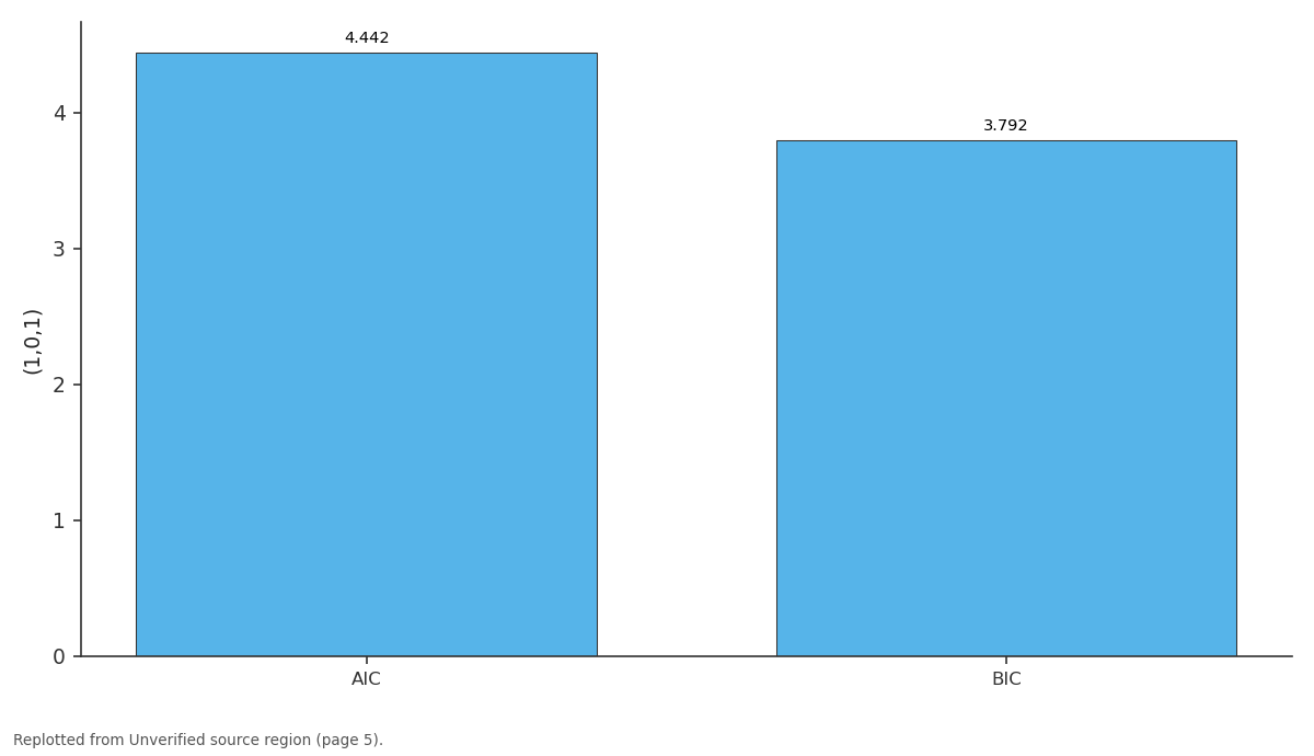
(1,0,1): AIC vs BIC
Replotted from a table (page 5) of the original paper. Every bar is the paper's own table value.
View source evidence ↗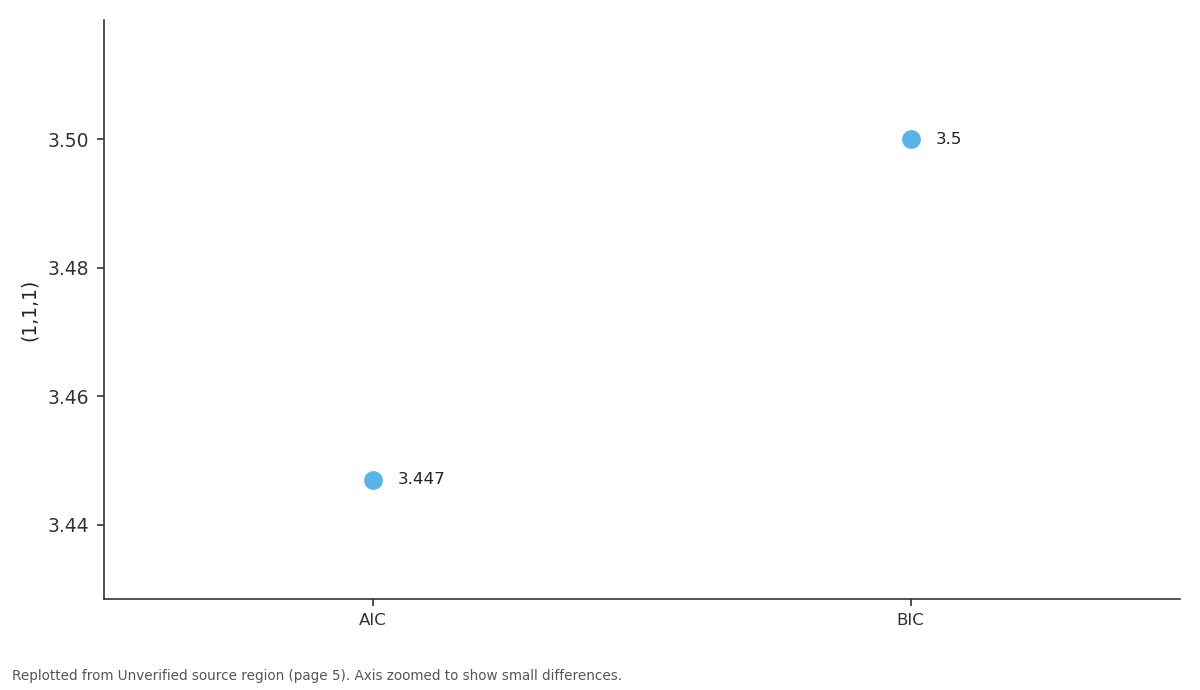
(1,1,1): AIC vs BIC
Replotted from a table (page 5) of the original paper. Every bar is the paper's own table value.
View source evidence ↗Figures & tables
From the original paper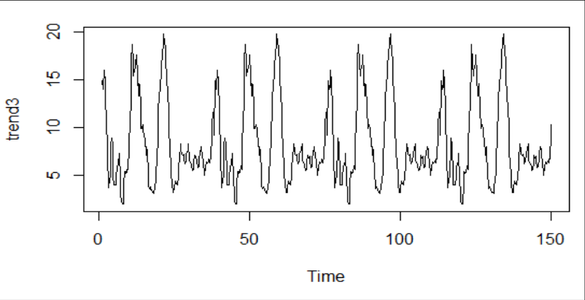 Figure 1
Introduction
Inflation is the general rise in the average level of a group of prices in a country. Inflation creates a problem because the purchasing power of money falls as the price level rises. It imposes an opportunity cost on holders of money. Inflation retards economic growth because the economy needs a certain level of savings to finance investments which boosts economic growth. Inflation causes global concerns because it can distort economic patterns and can result in the redistribution of wealth when not anticipated. Inflation can also discourage investors within and without the country by reducing their confidence level in investments. This is because investors expect high possibility of returns so that they can make good financial decisions. The maintenance of price stability is one of the macroeconomic challenges that the Kenyan government has been facing since its independence which is now 54 years ago. Inflation Rate in Kenya averaged 10.44 percent from 2005 until 2016, reaching an all-time high of 45.98% in 1993, 31.50% in May of 2008 and a record low of -0.1 in 1964 (KNBS,2016). Inflation modelling is one of the most important research area in monetary planning. According to Kohn, (2005):"Nothing is more important to the conduct of monetary policy than understanding and predicting inflation. Achieving and maintaining price stability will be more efficient and effective the better we understand the causes of inflation and the dynamics of how it evolves". Financial and economic models are heavily influenced by time, through both time resolution and time horizon. The resolution concept that signifies how densely data are recorded varying from seconds to years and time horizon looks at the length of time the data spans. Financial analysis usually involves a study of price movement, usually given over time, hence financial modelling focuses on building mathematical and statistical models to capture the price movements and the variations in the prices over time. Most economic and financial data are either non-linear or non-stationary, which is a problem when using the traditional statistical methods such as method of Box-Jenkins ARIMA models. It is necessary to look for other methods which are more appropriate and produce more accurate forecasts when the data is non-linear or non-stationary. In this study we will apply the method of autoregressive conditional heteroscedasticity ARCH as modern method of forecasting technique and see how it could be used as an alternative method to traditional methods. This technique showed in some studies in the last years that it can used efficiently in prediction in many subjects. In the present study we are going to perform some comparisons among GARCH and ARIMA models.
Literature Review
Review of inflation modelling Iqelan, B. M. (2015) [18] modelled the average monthly temperature data of Jerusalem in Palestine for the period from January 1964 to December 2013 using the ARIMA and GARCH modelling techniques to fit a historical data set and estimate the coefficients of the suitable models for fitting. The analysis of this study was carried out using the R software. Eventually, using different statistical measures, comparison efficiency between ARIMA (2, 0, 0) (3, 1, 1)12 and AR(1)-GARCH(1, 1) models were produced. AR (1)-GARCH(1,1) was found to be superior than ARIMA(2, 0, 0)(3, 1, 1)12 model. Yaziz, et.al. (2011), conducted a study to obtain a suitable GARCH and Box-Jenkins model for forecasting crude oil prices. ARIMA(1, 2, 1) and GARCH(1, 1) were found to be the appropriate models under model identification, parameter estimation, diagnostic checking and forecasting future prices. Comparison performances between ARIMA (1, 2, 1) and GARCH (1, 1) models ware made using several measures. GARCH(1, 1) was found to be a better model than ARIMA(1, 2, 1) model because the values for RMSE, Amos, (2009) studied financial time series modelling using inflation data spanning from January 1994 to December 2008 for South Africa. This study used the seasonal autoregressive integrated moving average SARIMA model and the generalized autoregressive conditional heteroscedasticity GARCH model which were fitted to the data for encountering trend and seasonal terms and accommodating time varying variance respectively. A best fitting model for each family of models offering an optimal balance on goodness of fit was selected. SARIMA(1, 1, 0)(0, 1, 1) and GARCH(1, 1) models were chosen to be the best fitting models for determining the two years forecasts of inflation rate of South Africa. However GARCH (1, 1) model was observed to be superior in producing future forecasts because of its ability to capture variations in the data. Chatfield, (2000); explored in his book that, the idea behind GARCH model is similar to that behind ARMA model in the sense that a higher order AR or MA model may often be approximated by a mixed ARMA model, with fewer parameters, using a rational polynomial approximation. Thus a GARCH model can be thought of as an approximation to a higher-order ARCH model. GARCH(1,1) model has become the standard model for describing changing variance for no obvious reason other than relative simplicity. In practice, if such a model is fitted to data, it is often found that (α + β) < 1 so that the stationarity condition may be satisfied. If α + β = 1, then the process does not have finite variance, although it can be shown that the squared observations are stationary after taking first differences leading what is called an integrated GARCH or IGARCH model. Akaike (1974) [1] and Schwarz (1978) developed Akaike Information Criterion (AIC or AICc) or the Bayesian Information Criterion (BIC). This will be used to select the final model. According to Hurvich and Tsai (1989), the AICc has a small sample size correction for the AIC and also converges to AIC in large samples. AIC and BIC are penalty statistic function used to measure goodness of fit of an estimated statistical model. Several competing models are developed and ranked according to the AIC, AICc or BIC and the one with the lowest information criterion value is chosen as the best. The information criteria idea is based on the extent to which the fitted values of the model approximate the true values. The penalty aspect discourages over fitting of the models so penalty increases with the number of estimated parameters. The AIC, AICc and BIC are computed as follows:
Methodology Seasonal Auto-Regressive Integrated Moving Average model (SARIMA)
The Box-Jenkins ARIMA model is generalized into a Seasonal Autoregressive Integrated Moving Average (SARIMA) model that accounts for both seasonal and non-seasonal characterized data. The SARIMA model is derived from the ARIMA model described above and also uses information on past observations and past errors of the series. Since the ARIMA model is inefficient for those series with both seasonal and non-seasonal behaviour for example in terms of wrong order selection, the SARIMA model is preferred when any seasonal behaviour is suspected in the series. The SARIMA model also sometimes referred to as the Multiplicative Seasonal Autoregressive Integrated Moving Average model, is denoted as ARIMA (p,d,q) (P,Q,D)s.
The corresponding lag form of the model is:
This model includes the AR and MA characteristic polynomials in L of order p and q respectively:
Also Seasonal polynomial functions of order P and Q respectively as represented below
Identifying the Seasonal ARMA Model
For pure SAR models, the autocorrelation function dies down and the partial autocorrelation function cuts off after one seasonal lag for a SAR (1) model. Similarly the partial autocorrelations die down for SMA models. Also the autocorrelation function cut off after one seasonal lag for SMA (1) model and after two seasonal lags for SMA (2). For the mixed seasonal ARMA with one SAR and one SMA both the autocorrelation function and partial auto correlation functions die down. The table below gives the summary of the stationarity and invertibility conditions of some specific seasonal time series models and the behaviour of their theoretical ACF and PACF.
Forecasting using the SARIMA model
Simple SARIMA model like SARIMA (0, 1, 1) (1,0,1)12 will be used to demonstrate how forecasts are obtained from the selected SARIMA model. Cryer and Chan (2008) demonstrated these steps below:
This pattern goes on, the residual terms 1 2 1 3 , , ...........
will be included in the first thirteen forecasts after which the AR part of the model takes over and produces the l >13 steps ahead forecasts in equation 5.7 below. The GARCH (p, q) model The Generalized ARCH (GARCH), as developed by Bollerslev, (1986) [5] , is an extension of the ARCH model similar to the extension of an AR to ARMA process. The GARCH (p, q) model employs the same equation as ARCH (1,1) for the log-returns 𝑦 𝑡 but the equation for the volatility, includes q new terms, that is
Where now 𝑡 > max (𝑝, 𝑞) and the remaining components are as in the ARCH model. The parameters of the model are for some positive integers. We see that if p=0 then the above model is reduced to the ARCH (q). Thus the GARCH model generalizes the ARCH by introducing values of 𝜎 𝑡-1 2 , 𝜎 𝑡-2 2 , …. in the equation: Let {𝑦 𝑡 } be the mean corrected return, 𝜀 𝑡 be a Gaussian white noise with mean zero and unit variance. Let also 𝐻 𝑡 be the information set or history at time t given by 𝐻 𝑡 = {𝑦 1 , 𝑦 2 , … , 𝑦 𝑡-1 } as in the ARCH model. Then the process { 𝑦 𝑡 } is GARCH (
Results and Discussions
In this study, a total of 150 monthly inflation data series (month on month-%) is used from January 2005 to December 2016 of month frequencies as they are in Nation Bureau of statistics of Kenya. The analysis was carried out using R statistical software. The ARCH type family models were fitted and forecast to the data because data was characterized by variation in variance and mean. The outcome of the study revealed that the ARCH -family type models, particularly, the EGARCH (1, 1) with generalized error distribution (GED) was the best in modelling and forecasting Kenya's monthly rates of inflation. It is revealed from figure 1 above that inflation rate for the period of 2005 to 2016 is non-stationary due to an unstable mean which increase and decrease at certain points. The mean and variance ought to be adjusted to form stationary series, so that the values vary more or less uniformly about a fixed level over time. The mean is not constant throughout the series as it assumes a downward trend by decreasing from the highest peak to the lowest peak.
The graph above indicates that in the time series there seems to be seasonal variation in the inflation rate. Again, it seems that this time series could probably be described using an additive model, as the seasonal fluctuations are roughly constant in size over time and do not seem to depend on the level of the time series, and the random fluctuations also seem to be roughly constant in size over time.
Below is the summary of the above trend To confirm the presence of stationarity, the Augmented Dickey-Fuller (ADF) test was performed. The test fails to reject the null hypothesis of unit root at 5% level of significance and thus it can be concluded that the rate of inflation is not stationary. For this purpose, a first order lagged difference from the original series is obtained. Augmented Dickey-Fuller (ADF) test is conducted on this series to check for stationarity. The ADF test shows that the series is stationary. The t-statistic of -6.607 and -6.628 is smaller than 1% of test critical value. The p-value for ADF test is zero indicating that we have sufficient evidence to reject the null hypothesis of the series being non-stationary.
ARIMA model Model selection on ARIMA
The study sought to determine the best ARIMA model and the most suitable GARCH model. Series: my time series ARIMA (2,0,0)(0,0,1) [12] The creation of the ARIMA model for the data in R is done using the r package forecast and forecast library. However if you want to choose the model yourself, use the Arima () function in R till you get the minimum AICc value which is considered to be the best model. The auto. arima () function is used to determine the best ARIMA model automatically from R as shown below;
The above model was selected using stepwise selection criterion based on the Akaike Information Criterion corrected (AICc). This is a seasonal ARIMA model which sometimes referred as SARIMA. Therefore, since the seasonal ARIMA is the best forecasting equation, it means that inflation is affected by the periodic calendar. This is shown in the trend (the trend mimics a sine function). The model parameters are; AR1 which stands for non-seasonal autoregressive component of order 1, AR2 refers to the non-seasonal component of order 2 and sma1 refers to the seasonal simple moving average of order 2.
The best ARIMA model to be used for that data is ARIMA (2,0,2) Plots Call: Garch (x = Data$inflation. rate, trace = FALSE) Coefficient(s): a0 a1 b1 1.746e+ 01 9.317e-01 4.690e-13 The two models (for the conditional mean and the variance) are perfectly compatible with each other, in that the mean of the process can be modelled as ARMA, and the variances as GARCH. This leads to the complete specification of an ARMA (p,q), GARCH(r,s) model. ARMA is a model for the realizations of a stochastic process imposing a specific structure of the conditional mean of the process. GARCH is a model for the realizations of a stochastic process imposing a specific structure of the conditional variance of the process. However in our case we are interested in forecasting the inflation rates in Kenya than comparing their volatility thus the ARIMA (2,0,2) will be our best model in forecasting our results as below. Forecasting the inflation using ARIMA (2, 0, 2)
The trend shows the normal seasonal variations of the inflation rates, however the forecast indicate a continued increase in the inflation in the future as illustrated by the figure above.
GARCH Model Model selection and analysis
The idea of the research is to have a good model that captures as much variation in the data as possible. Usually the simple GARCH model captures most of the variability in most stabilized series. Small lags for p and q are common in applications. Some models are typically adequate in different study such as GARCH (1, 1); GARCH (2, 1) or GARCH (1, 2) models for modelling volatilities even over long sample periods (Bollerslev, Chou and Kroner, 1992). However in the table below the GARCH (0, 1); GARCH (0; 2) and GARCH (2; 2) has been included in order to check if they are appropriate for modelling time varying variances of the data. The smaller the AIC and BIC the better. Larger AICs; BICs and standard error makes the model unfavorable. The table above shows the competing models to the data with their respective AIC; BIC and SE: From the derived models using the method of maximum likelihood, the estimated parameters of the models with their corresponding standard error and other statistical tests.
Comparison of suggested GARCH models
Comparison of suggested GARCH models
Model
The standard errors are used to assess the accuracy of the estimates, the smaller the better. The model fit statistics used to assess how well the model fit the data are the AIC and BIC: The corresponding values are: AIC = 5.127 and BIC = 5.019 with the log likelihood value of -465.23. The standard errors are quiet small suggesting precise estimates. Based on 95% confidence level, the coefficients of the GARCH (1; 1) model are significantly different from zero and the estimated values satisfy the stability condition.
Forecasting comparison using
Forecasting comparison using
References
21 in the original paper- Akaike H. A new look at the statistical model identification, IEEE transaction on automatic control. 1974; 19(6):719-723.
- Amos C. Time Series Modelling with Application to South African Inflation Data, A thesis submitted to University of Kwazulu Natal for the degree of Masters of Science in Statistics, 2010.
- Assis K, Amran A, Remali Y. Forecasting Cocoa Bean Prices Using Univariate Time Series Models, Journal of Arts Science and Commerce, 2006. ISSN 2229 -4686.
- Assefa Y. Time Series and Spatial Analysis of Crop Yield, M.Sc. KANSAS STATE UNIVERSITY, Manhattan, Kansas, 2013,
- Bollerslev T. Generalized autoregressive conditional hetroscedasticity. Journal of Econometics. 1986; 31:307-327.
- Bollerslev TRY, Chou, Kroner KF. ARCH Modelling in Finance: A Selective Review of the Theory and Empirical Evidence, Journal of Econometrics. 1992; 525-59.
- Bollerslev T. Volatility and Time Series Econometrics: Glossary to ARCH (GARCH).Essays in Honour of Robert F. Engle. Oxford University press, 2009.
- Box G, Jenkins G. Time Series Analysis, Forecasting and Control, Holden Day, San Francisco, 1976.
- Brockwell PJ, Davis RA. Introduction to Time Series and Forecasting, 2nd Edition. Springer, New York, 2002.
- Chatfield C. Time Series Forecasting: University of Bath, Chapman and Hall text in statistical science, London, 2000,
- Charline Uwilingiyimana, Joseph Munga'tu, Jean de Dieu Harerimana. Forecasting Inflation in Kenya Using Arima -Garch Models. International Journal of Management and Commerce Innovations. 2016, 15-27.
- Cryer JD, Chan KS. Time Series Analysis With Applications in R. Springer, 2nd Edition U.S.A, 2008
- Edward N. Modelling and Forecasting Using Time Series GARCHModels: An Application of TANZANIA Inflation Rate Data, M.Sc. Mathematical Modelling Dissertation, University of Dar es Salaam, 2011.
- Engle R. The USE of ARCH/GARCH Models in Applied Econometrics; Journal of Economic Perspectives 1982; 15(4):157168.
- Engle RF. Autoregressive conditional heteroscedastisity with estimates of the variance of United Kingdom inflation Econometrics. 1982; 50:987-1007.
- Engle RF, Bollerslev T. Modeling the persistence of conditional variances, Econometric Reviews. 1986; 5:1-50.
- Garcia RC, Javier C, Marko A, Garcia BS. A GARCH Forecasting Model to Predict Day-Ahead Electricity Prices, A paper submitted to the IEE power system Journal in Berlin, 2003.
- Iqelan BM. Time Series Modelling For Monthly Temperature Data Of Jerusalem/Palestine. Matematika, UTM Centre for Industrial and Applied Mathematics, 2015; 31(2):159-176.
- Suhatono. Time Series Forecasting by using Seasonal Autoregressive Integrated Moving Average: Subset, Multiplicative or Additive Model,Journal of Mathematics and Statistics. 2011; 7(1):20-27.
- Tsay RS. Analysis of Financial Time Series. 2002, ISBN 0-471-41544-8
- Tsay RS. Analysis of Financial Time Series, 2nd edition, New Jersey, University of Chicago, John Wiley Sons, 2005, 22. Yaziz SR, Ahmad MH, Nian LC, Muhammad N. A Comparative Study on Box-Jenkins and GARCH Models in Forecasting Crude Oil Prices, Faculty of Industrial Sciences and Technology, University of Malaysia Pahang, 2011.
Cited by 1
From OpenAlex, OpenCitations and reference lists read by Scinovex
- Mathematics Model on Syariah Share Pricing in ISSI ↗
Padrul Jana, Anindita Imam Basri · Jurnal Derivat Jurnal Matematika dan Pendidikan Matematika · 2020
The ability to read, analyze data, and execute the Syariah economic market agents' decision becomes possible to happen. This research aims to help agents and those how to read the data, analyze, and model the data by providing perspectives regarding the stock pricing in the future. The research method being employed as Autoregressive Integrated Moving Average (ARIMA), which has steps…
❝ 0PDF