
Research article · 2019 · Full text
International Journal of Statistics and Applied MathematicsANOVA in GLS transform vs. Welch’s ANOVA under heteroscedasticity
Volume 4(1) · Pages 62–65
Research areasStatistical Distribution Estimation and Applications
Abstract
Author-writtenHeteroscedastic data arise from a population whose sub-populations have different variabilities from one another. In presence of heteroscedasticity, the LS estimators no longer remain the BLUEs, giving rise to wider acceptance regions and confidence intervals for the model parameters. The most conventional way of removing heteroscedasticity is the generalized least square technique. One can perform one-way ANOVA on this transformed data or use Welch’s ANOVA. This paper compares the efficiencies, i.e., the power of these two methods.
Summary
Source-checkedPlain-language reading of the full paper, prepared with AI and checked against the text. Each point links to the authors' own words.
Why it matters
- Heteroscedasticity occurs when different sub-populations within a dataset exhibit different levels of variability. View evidence ↗
- When heteroscedasticity is present, Least Squares (LS) estimators are no longer the Best Linear Unbiased Estimators (BLUEs), which results in wider confidence intervals and acceptance regions. View evidence ↗
- The generalized least square (GLS) technique is a standard method used to remove heteroscedasticity from data. View evidence ↗
The question
- The study aims to compare the efficiency, specifically the statistical power, of performing one-way ANOVA on GLS-transformed data versus using Welch's ANOVA. View evidence ↗
What they did
- The researchers used the 'Engel data' from R, which contains 235 observations of food expenditure and income for Belgian working-class households. View evidence ↗
- The income variable was converted into a categorical variable with three levels: low, middle, and high income groups. View evidence ↗
- The assumption of equal variance for ANOVA was violated, as standard deviations for food expenditure varied from 75.83375 (low income) to 282.972 (high income). View evidence ↗
- Using Glejser's test, the authors determined that the standard deviation is proportional to income (σi xi) based on the maximum t-value at δ2* = 1. View evidence ↗
- GLS transformation was applied by dividing the response variable (y) by the explanatory variable (x). View evidence ↗
What they found
- After GLS transformation, the variances across the three income groups became nearly equal, approximately 0.085. View evidence ↗
- One-way ANOVA on the transformed data rejected the null hypothesis of equal means for food expenditure across the three income groups at 95% confidence. View evidence ↗
- Welch's ANOVA also rejected the null hypothesis with an observed Fw of 194.41 and a p-value less than 2.2e-16. View evidence ↗
- The statistical power for the ANOVA on transformed data was calculated as 0.998. View evidence ↗
- The statistical power for Welch's ANOVA was calculated as 1. View evidence ↗
- While Welch's ANOVA produced a significantly lower p-value than the classical ANOVA on transformed data, the statistical power of both methods was nearly identical. View evidence ↗
What it means
- The authors conclude that both GLS-transformed ANOVA and Welch's ANOVA are highly useful as they yield consistent results. View evidence ↗
- The authors state that Welch's ANOVA is superior to GLS-transformed ANOVA because it does not lose the original data, making interpretation easier. View evidence ↗
Visual summary
1 visualsIllustrations explain the paper; they do not show study data.
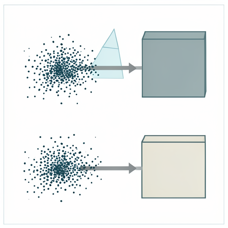
Comparison of ANOVA Workflows
AI-generated conceptual illustration (Abstract mathematical data representations as colored scatter plots). It explains the idea and does not show study data.
View source evidence ↗Figures & tables
From the original paper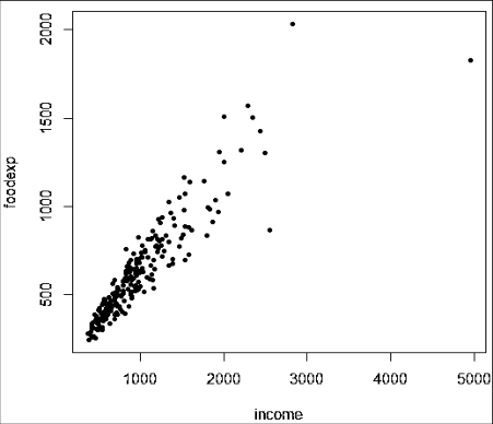 Figure 1
 Table 1
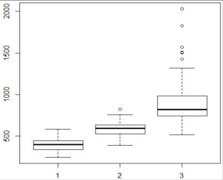 Figure 2
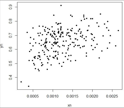 Figure 3
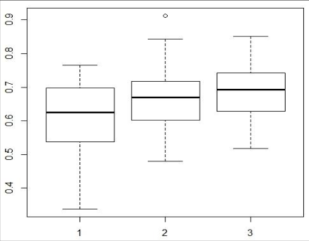 Figure 4
 Table 2
Introduction
Let us consider the dataset named "Engel data" from R, consisting of 235 observations on income and expenditure on food for Belgian working class households (Belgian Francs). The scatterplot, obtained from R, is given below. The scatterplot in Figure 1 shows that as income increases, the expenditures of the Belgian workers become more dispersed, suggesting the presence of heteroscedasticity. We now create a new column in "Engel" that converts the variable "income" into a categorical variable called "inc_gr" with three levels called "1", "2", and "3", denoting the low income group, the middle income group and the high income group. The lowest third of the data belongs to the first level, the middle third belongs to the second level, and the highest third of the data to the third level. This is done by dividing the variable "foodexp" into three parts as per their quantiles corresponding to 0.333 and 0.666.
[R] Code Quantile (engel $income, seq (0, 1, 1/3)) inc_gr = cut (engel $income, c (377, 718.3701, 1014.1540, 4958), labels = c (1, 2, 3)) Engel = cbind (engel, inc_gr)]
The assumptions of the one-way analysis of variance are 1. The data are continuous (not discrete). 2. The data follow the normal probability distribution. Each group is normally distributed about the group mean. 3. The variances of the populations are equal. 4. The groups are independent. There is no relationship among the individuals in one group as compared to another. 5. Each group is a simple random sample from its population. Each individual in the population has an equal probability of being selected in the sample.
On checking the variance or standard deviation of food expenditure corresponding to the three income groups, we fing them to differ widely; SD of food expenditure for lower income group is 75.83375, SD of food expenditure of middle income group is 89.53907 and that for the high income group is 282.972 Hence, the assumption of ANOVA is violated. The two remedies in such situations are stated next.
[R] Code Plot (engel $inc_gr, engel $ foodexp, type = "p")]
Materials and Methods
Materials and Methods
Generalised Least Square Method
If the true nature of σ i 2 is known, then, the GLS technique [1,2] converts the heteroscedastic error to homoscedastic error, i.e., σ i 2 = σ 2 i, by dividing the model by the known standard
The estimates of β 1 and β 2 obtained by the method of least squares with the transformed data on this new model are the generalized least square (GLS) estimates. In our case, and in most practical cases, the true nature of σ i 2 remains unknown. We seek help of the Glejser's test [3,4] to identify the nature of σ i 2 and then GLS method is applied as before.
Here, we consider the model x .
For the engel data, we get As we can see from Table 1, the modulus of t-value for δ 2 * = 1 is maximum and therefore is considered to be the most significant. We thus conclude that σ i x i .
| δ2* | -1 | -½ | ½ | 1 |
|---|---|---|---|---|
| |t-value| | 6.624 | 7.95 | 11.704 | 13.981 |
| p-value | 0.00 | 0.00 | 0.00 | 0.00 |
Table text extracted from the original PDF; superscript letters are shown inline. The original table image is below.
View original table image
The transformed data is obtained as y n = y/x and x n = 1/x. The scatterplot of the transformed data isClearly, the scatterplot shows no more sign of any heteroscedasticity. The transformed data thus satisfies all conditions required for conducting a one way ANOVA.
The transformed response variable y n now has almost equal variances (close to 0.085) in the three groups. This is further represented by a boxplot below. The transformed data is now suitable for the one way ANOVA test. We obtain the ANOVA table through the lm (.) function in R. We reject the null of equal means (average food expenditure for all the three income groups are same) with 95% confidence. Now we check the power of this ANOVA test [5,6] . The power of any test of statistical significance is defined as the probability that it will reject a false null hypothesis.
Statistical power is inversely related to beta or the probability of making a Type II error. In short, power = 1-β.
In other words, statistical power is the likelihood that a study will detect an effect when there is an effect there to be detected. If statistical power is high, the probability of making a Type II error, or concluding there is no effect when, in fact, there is one, goes down. Statistical power is affected chiefly by the size of the effect and the size of the sample used to detect it. Bigger effects are easier to detect than smaller effects, while large samples offer greater test sensitivity than small samples. The ANOVA model is (y n ) it = μ i + ε it ; i = 1,..,p ; t = 1(1)n [Here p=3, n=78] where ε it are i.i.d N(0,σ 2 ). To test the hypothesis that the treatment means are all equal, we use F = MST/MSE (the ratio of the mean square between groups to the mean square within groups) and reject the null hypothesis if F obs > F 2, 232, α for a given probability of type I error α. When the null hypothesis of mean equality is rejected, the above ratio has a non-central F distribution which adds a noncentrality parameter [7] , λ. This parameter is calculated as
(weighted mean of all groups). Cohen (1988) [8] proposed an effect size parameter f which he defined as f 2 = 𝜎 𝑚 2 𝜎 2 . Using this, the non-centrality parameter reduces to 𝜆 = f 2 ∑ 𝑛 𝑖 𝑝 𝑖=1 . Now, another effect size is given by
1+𝑓 2 , which is the proportion of the total variation in the dependent variable that is attributable to the groups. The power is computed as the probability of being greater than F p1, p(n-1) , α on a noncentral-F distribution with non-centrality parameter λ, where λ is calculated from 𝜂 2 using the formula given above. In our example, we get the effect size as Using R software, we compute power with the command pwr. ANOVA. Test (k=3, n=78, f=0.386279, sig. level=0.05) and obtain the power as 0.998.
Welch's ANOVA
For testing the equality of k sample means, when the variances are not equal, Welch (1951) [9][10][11] provided the following modification of the usual ANOVA F-test:
Results and Discussions
We observe that both one way ANOVA on transformed data and Welch's ANOVA test for the engel dataset gives the same decision, i.e., rejecting the null hypothesis of equal means of expenditure for food. The p-value for Welch's ANOVA test is much less than that of the classical one way ANOVA test, however power remains more or less same. As such, no discrepancy is noticed between the two results, which establishes the immense utility of both the methods. One drawback of the classical one way ANOVA on the GLS transformed data is that the original data is lost and all results are based on a completely new data set obtained by dividing the original data by the explanatory variable. This creates difficulty in proper interpretations. The Welch's ANOVA surpasses the one way ANOVA on this ground.
Figures and tables from the paper
| Source | df | SS | MS | F | p-value |
|---|---|---|---|---|---|
| Income group | 2 | 0.26646 | 0.133232 | 17.301 | 9.916e-08 |
| Error | 232 | 1.78656 | 0.007701 | ||
| Total | 234 | 2.05302 | - |
Table text extracted from the original PDF; superscript letters are shown inline. The original table image is below.
View original table image
References
11 in the original paper- Damodar NG. Heteroscedasticity. In: Basic Econometrics. Fourth edition, The McGraw-Hill Companies, US, 2004, 387-426.
- Qingfeng L, Ryo O, Arihiro Y. Generalized Least Squares Model Averaging. Econometrics Reviews. 2016; 35(8-10):1692-1752.
- Edgar PH, Clayton SL. A note on glejser's test for heteroscedasticity. Communications in Statistics. 1980; 9(12):1209-1220.
- Jose AFM, Santos Silva JMC. Glejser's test revisited. Journal of Econometrics. 2000; 97(1):189-202.
- Joel RL. Overcoming Feelings of Powerlessness in "Aging" Researchers: A Primer on Statistical Power in Analysis of Variance Designs, Psychology and Aging. 1997; 12(1):84-106.
- Wilcox RR. ANOVA: A paradigm for low power and misleading measures of effect size, Review of Educational Research. 1995; 65(1):51-77.
- Xiaofeng L, Stephen R. A Note on the Noncentrality Parameter and Effect Size Estimates for the F Test in ANOVA, Journal of Educational and Behavourial Statistics. 2004; 29(2):251-255.
- Joseph LG, Yulia RG, Weiwen M. The Impact of Levene's Test of Equality of Variances on Statistical Theory and Practice, Statistical Science. 2009; 24(3):343360.
- Mehmet M, Soner Y. Comparison of ANOVA-F and ANOM tests with regard to type I error rate and test power, Journal of Statistical Computation and Simulation. 2013; 83(11):2093-2104.
- Kenneth JL. An empirical comparison of the ANOVA Ftest with alternatives which are more robust against heterogeneity of variance, Journal of Statistical Computation and Simulation. 1978; 8(1):49-57.
- Mehmet M, Erkut A. Comparison of ANOVA F and Welch Tests with Their Respective Permutation Versions in Terms of Type I Error Rates and Test Power, Kafkas Universitesi Veteriner Fakultesi Dergisi. 2010; 16(5):711-716.