
Research article · 2018 · Full text
International Journal of Statistics and Applied MathematicsReconstructing earth observation vegetation index records with a Bayesian spatiotemporal dynamic model
Volume 3(4) · Pages 74–84
Research areasRemote Sensing in AgricultureSpecies Distribution and Climate ChangeSoil Geostatistics and Mapping
Abstract
Author-writtenLong-term vegetation index records derived from Earth observation facilitate the characterization of ecosystem response to climate variability and change. The presence of atmospheric components and radiometric inconsistencies lead to gaps and artificial jumps in the time series, making such characterization difficult. Compositing over days or weeks minimizes these effects to some degree, but further processing is often performed. In this paper, we develop a spatiotemporal dynamic linear model (DLM) that produces more consistent vegetation index data, while preserving adequate temporal resolution to support accurate global change research. The technique takes the stochastic partial differential equations (SPDE) approach, but employs the Integrated Nested Laplace Approximation (INLA) to decrease computational demand. The new routine was tested on the monthly Vegetation Index and Phenology (VIP) Lab Enhanced Vegetation Index-two (EVI2) version 3 products at 10 km resolution. VIP-EVI2 is derived from red and near-infrared top of atmosphere reflectance, which is measured by the Advanced Very High Resolution Radiometer (AVHRR) on board several National Oceanic and Atmospheric Administration satellites. Performance of the procedure was compared to an adaptive Savitzky-Golay (S-G) filter, forward filtering and backward sampling (FFBS), and a spatiotemporal dynamic model based on a Gibbs sampler. The inter-comparison was made by descriptive analysis, cross-validated root mean squared error, and generalized coefficient of efficiency. Overall, the SPDE showed a higher level of fidelity compared to the alternative techniques. If computational resources are not heavily restricted, the new gap-filling and smoothing procedure provides a viable alternative to standard routines.
Summary
Source-checkedPlain-language reading of the full paper, prepared with AI and checked against the text. Each point links to the authors' own words.
Why it matters
- Long-term vegetation index records from Earth observation are important for understanding how ecosystems respond to climate change and variability. View evidence ↗
- Atmospheric components and radiometric inconsistencies create gaps and artificial jumps in these records, which hinders the characterization of ecosystem responses. View evidence ↗
- Persistent cloud cover in tropical regions leaves significant gaps in the data, reducing the sample sizes needed for statistically precise global and regional change studies. View evidence ↗
The question
- The study aims to demonstrate that a full Bayesian spatiotemporal dynamic linear model (DLM) provides more robust, consistent, and precise projections for missing data in VIP-EVI2 records than alternative methods. View evidence ↗
What they did
- The researchers tested their routine using monthly VIP-EVI2 version 3 products at a 10 km spatial resolution. View evidence ↗
- The study area was subset to Kenya, specifically between latitudes 33.6° and 42° and longitudes -4.8° and 5.8°. View evidence ↗
- The proposed method was compared against an adaptive Savitzky-Golay (S-G) filter, forward filtering and backward sampling (FFBS), and a spatiotemporal dynamic model using a Gibbs sampler (DLM-MCMC). View evidence ↗
- The techniques were compared using descriptive analysis, cross-validated root mean squared error (RMSE), and the generalized coefficient of efficiency (E). View evidence ↗
What they found
- The spatiotemporal DLM-SPDE approach produced means and standard deviations that were closer to the good-quality data than the adaptive S-G and FFBS methods. View evidence ↗
- The adaptive S-G and FFBS routines generally showed higher root mean squared error (RMSE) across pixels than the spatiotemporal DLM procedures. View evidence ↗
- The spatiotemporal DLM-SPDE was the only method that maintained a very high generalized coefficient of efficiency (E) at tropical latitudes. View evidence ↗
- The lowest RMSE was achieved by the spatiotemporal DLM-MCMC and DLM-SPDE, with fewer than 10% and 1% of pixels recording an RMSE greater than 0.1, respectively. View evidence ↗
- More than 90% of the pixels processed with the spatiotemporal DLM-SPDE resulted in a generalized coefficient of efficiency (E) greater than 0.7. View evidence ↗
- Unlike the spatiotemporal DLM-MCMC and DLM-SPDE, the FFBS and adaptive S-G methods were significantly affected by low sample sizes (low percentage of available data before processing). View evidence ↗
What it means
- The authors recommend using FFBS if computational resources are highly restricted, due to its efficiency and relatively high accuracy. View evidence ↗
- The authors suggest that future work could employ more stable model calibration and validation rules, such as 10-fold cross-validation, to improve the evaluation of prediction quality. View evidence ↗
Visual summary
1 visualsIllustrations explain the paper; they do not show study data.
Comparison of Vegetation Index Reconstruction Methods
AI-generated conceptual illustration (Satellite-observed vegetation indices of a mixed forest landscape). It explains the idea and does not show study data.
View source evidence ↗Figures & tables
From the original paper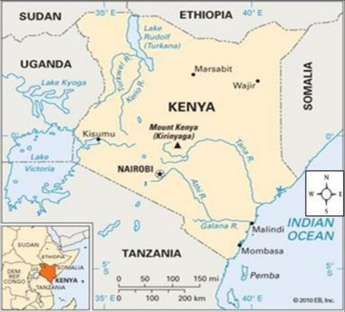 Figure 1
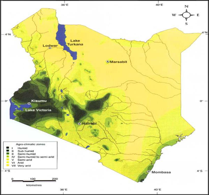 Figure 2
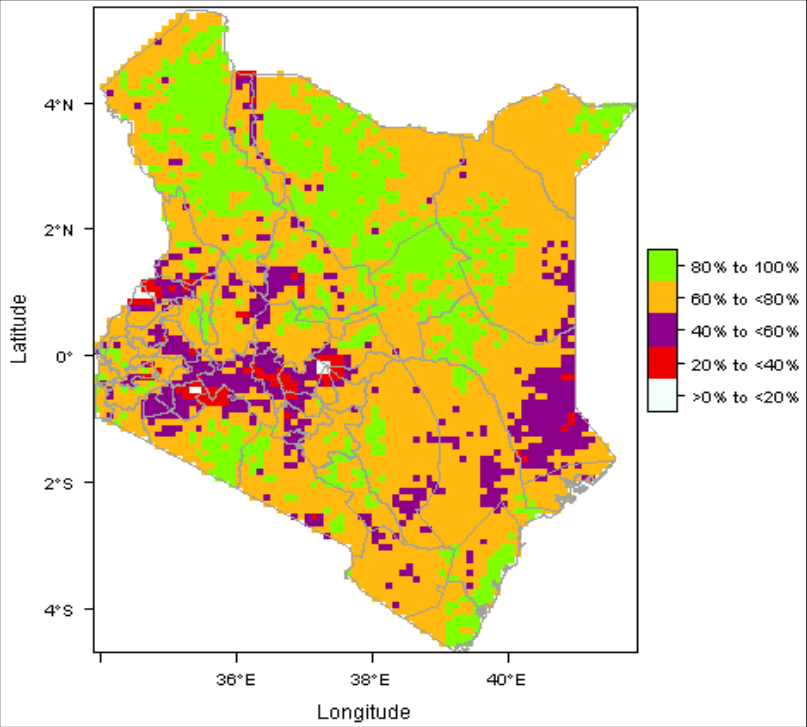 Figure 3
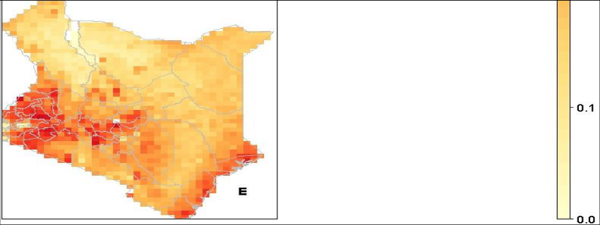 Figure 4
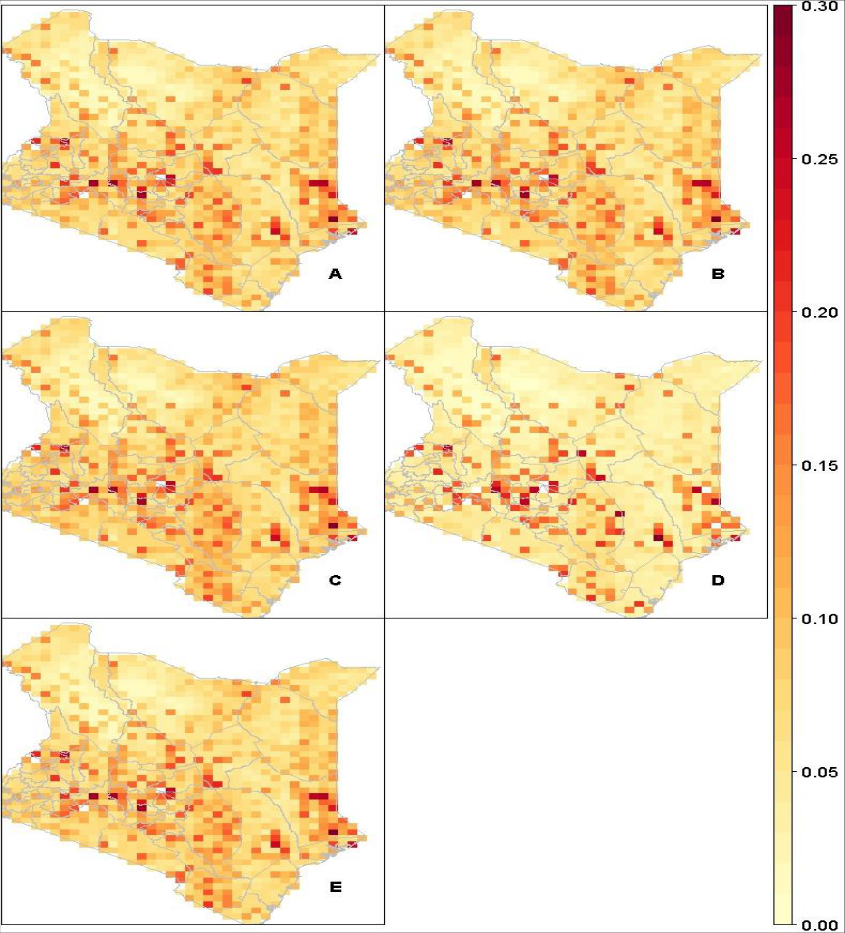 Figure 5
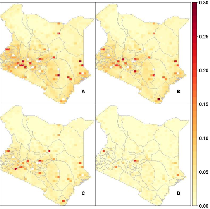 Figure 6
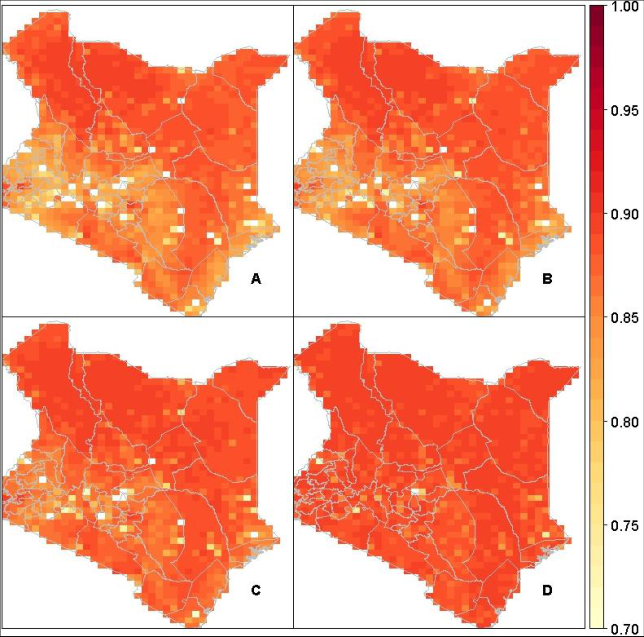 Figure 7
Introduction
Over three decades of daily Earth observation vegetation index records are currently available for a wide range of climate and environmental research and applications (Beck et al., 2011) [6] . However, gaps and inconsistencies within the records limit their usefulness for such research and applications (Vermote et al., 1994) [36] . Daily data has been composited to weekly or bimonthly time-steps (Holben, 1986) [19] to improve continuity and reduce noise. Even so, gaps remain, particularly in tropical regions with persistent cloud cover, significantly reducing sample sizes necessary to achieve statistical precision for accurate assessment of global and regional change studies necessitating further processing by reconstruction (Barreto-Munoz, 2013) [5] . Adaptive Savitzky-Golay (S-G), forward filtering and backward sampling (FFBS) are two of the most commonly used gap-filling and smoothing procedures in remote sensing. Conceptually, adaptive S-G utilizes a piece-wise polynomial regression with optimized pixellevel smoothing parameters (polynomial order and window length) which is critical when the data have no smooth trend (e.g. sinusoidal). Unlike the adaptive S-G, FFBS is a state-space approach with model parameters evolving smoothly over time. Vivar and Ferreira (2009) [37] suggested the FFBS algorithm to circumvent the strong autocorrelation of the recursions and chains that Kalman-Filtering and Markov Chain Monte-Carlo (MCMC) algorithms are known to suffer while sampling from a dynamic process. Generally, both the adaptive S-G and FFBS are curve fitting techniques except that while the former operate on local (piece-wise) window, the latter considers whole (global) window adopting state-space procedure for the dynamic attributes characterized with vegetation index records. When the underlying process of long-term vegetation time series records is dynamic, reconstruction must be done in a probabilistic way (Weiss et al., 2014) [39] . This is naturally handled with hierarchical Bayesian modelling. Uncertainty regarding the true estimates of the pixel-level dynamic parameters is then expressed by appropriate probability distributions. However, due to computational bottleneck involving space-state attributes, reconstruction with such models have had many setbacks (West and Harrison, 1997) [40] . However, simulation and techniques based on numerical methods have been proposed in a bid to help end users benefit from methodological development of Bayesian dynamic linear models (DLMs). They include: generalized estimation equation (Zeger, 1988) [44] ; sequential estimation and discount factor approach to modelling of the unknown variances (Pole et al., 1994) [27] ; MCMC approach (Gamerman, 1998) [15] ; importance sampling for likelihood estimation and signal extraction (Koopman et al., 1999) [22] ; decomposition of time series and evaluating space-time using seasonal component based on maximum likelihood estimation (Ripley, 2002) [28] ; an iterated extended Kalman filter approach adaptive resampling scheme (Schmidt et al., 1999) [33] ; Laplace approximation (Gamerman, 1998) [15] among others. Recently, other developments have extended the Bayesian DLMs beyond temporal autocorrelations. For instance, Finley et al. (2007) [14] proposes a model consisting of space-time regression models with spatially varying coefficients for short length time series data, which has also been adopted in. However, the approach does not provide adequate temporal predictions making it less flexible for large scale spatiotemporal DLMs. Has proposed an alternative which utilizes the SPDE approach to obtain spatiotemporal inferences of model parameters using MCMC sampling technique. Even so, the approach does not allow spatial modeling with spatially varying coefficients processes limiting its application in spatio-tetemporal DLMs. A more flexible technique involving spatiotemporal inference using MCMC has also been proposed to fit spatially and temporally predict hierarchical Bayesian point-referenced space-time data (Bakar and Sahu, 2015) [4] . The flexibility of the technique by providing more flexible alternative sampling schemes (e.g. restricted maximum likelihood estimation, MCMC with Gibbs sampler etc.) that is desirable for complex models. This study considered the spatiotemporal DLM-MCMC to be comparable to the new method proposed, given that it also make use of Bayesian inferential procedure, expressng space-state parameters with Mate ˋrn covariance function and random walk 1 (Bakar et al., 2015b) [3] . According to Ruiz-Cárdenas et al. (2012) [32] , when the latent field is Gaussian, with observations already measured, and the interest is in the estimation of the dynamic parameters using the available information, Integrated Nested Laplace Approximation (INLA) can be adopted to approximate their marginal posterior distributions (Rue et al., 2009) [9] . We can also express spatial dependence structure of the underlying dynamic parameters with the stochastic partial differential equations (SPDE) approach (Lindgren et al., 2011) [24] . The model expression is fairly similar to that of DLM-MCMC. According to Held et al. (2010) [18] , if the MCMC sampling scheme converges to the target posterior distribution and the necessary INLA assumptions necessary for accurate numerical operations are satisfied, then the two models (DLM-MCMC and DLM-SPDE) should provide estimated and predicted values that are fairly similar. The DLM-MCMC involves dense covariance matrices which can result into intractability of the complex matrix algebra during computation as oppose to the sparse precision matrices associated with DLM-SPDE. Furthermore, the DLM-MCMC can pose a challenge in assessing pixel-level convergence to the target posterior/predictive distributions resulting in some cases to inference from a false positive distribution. The primary goal of this paper is to illustrate that full Bayesian spatiotemporal DLM provides more precise, consistent and robust projections of bad quality (missing) data in VIP-EVI2 records compared to other alternative techniques presented in this study. The spatial random field is expressed by SPDE model functionalities with the Matérn covariance function while the temporal evolution takes a RW1 process. The paper is organized as follows: In section 2.1, EVI2 is described; in sections 2.2-2.4, the SPDE approach, an adaptive S-G filter, FFBS, and spatiotemporal DLM with MCMC are briefly presented. An overview of the analytical and inferential procedures used to compare the performance of the techniques is provided in sections 2.5. Results of the inter-comparison are provided in section 3, followed by a discussion and conclusion in sections 4 and 5, respectively.
Data, Processing and Methods
Data, Processing and Methods
Vegetation Index & Phenology (VIP) Lab Version 3 Enhanced Vegetation Index 2 (EVI2)
We used the EVI2 record for comparison, given persistent data gaps that remained in the record after pre-processing. The VIP-EVI2 (Jiang et al., 2008) [20] is a multi-sensor product that fuses the Moderate-Resolution Imaging Spectroradiometer (MODIS) and Advanced Very High Resolution Radiometer (AVHRR). The original record is available globally at 15-day and 5km temporal and spatial resolutions respectively. The record was subset for Kenya, latitude between 33.6 o and 42 o and longitude between -4.8 o and 5.8 o (Figure 1). Monthly record was developed here from maximum of the bimonthly records averaged for four neighboring pixels to form a 10km spatial resolution. The downscaling was done so as to have a common platform for inter-comparison given computational challenges realized with spatiotemporal DLM-MCMC. Kenya was considered given the different agro-climatic zones and diverse land cover types that exist (Figure 2). In this way, potential effect of proximity to water body and mountain on the reconstruction techniques can be evaluated. The original record includes pixel reliability (PR) bands that characterize the surface reflectance state, condition of the atmosphere and other useful information about each pixel (Didan, 2014) [11] . PR is indexed from 0 to 7 denoting high to worst quality data respectively. EVI2 is derived from:
Where, NIR and RED are the Near Infrared and visible red energy reflected from the Earth's surface and received by the sensor. EVI2 ranges from +1.0 to -1.0. Areas of barren rock, sand, or snow usually show very low EVI2 values (e.g. 0.1 or less). Sparse vegetation such as shrubs and grasslands or senescing crops may result to moderate EVI2 values between 0.2 and 0.5.
Fig 2:
The Kenya agro-climatic zones with Lakes marked as blue while rivers and streams are marked as black.
Dense vegetation such as forest or peak farmland may result to high EVI2 values between 0.6 and 0.9. Pixel level data denoted by the PR index other than excellent or good (0 and 1 respectively) were classified as bad-quality data and shown as gaps in the records before downscaling, because pixels with PR > 1 are significantly affected by clouds, aerosols, dust, Rayleigh scattering, and other noise. This resulted in large, persistent and irregularly spaced data gaps, beyond the ability of some of the smoothing and gap-filling methods evaluated in this study. So, some gaps were filled before the assessment using a MODIS filtering algorithm.
Percentage of pixel level good quality records available before gap-filling and smoothing was evaluated given the statistical effect of sample size variability on the goodness-of-fit. From our estimation, about 15% of the pixels had <40% good quality data mostly concentrated in the high rainfall areas either neighboring a water body or a mountain, 45% of the pixels had between 40-60% good quality records, 35% of the pixels had between 60-80% good quality data while the remaining pixels (5%) had >80% good quality data of which over 50% were distributed around Lake Turkana as shown in Figure 3. The Vegetation Index & Phenology (VIP) Lab Version 3 Enhanced Vegetation Index 2 records tested in this study is hereafter referred to as VIP-EVI2.
Spatiotemporal DLM SPDE theoretical Basis with INLA
The simplest case of a space-state dynamic model using INLA is provided by a random walk order 1 (RW1) process. In this case, the observation equation can be written as shown in equation 2.
𝑦 𝑡 = 𝑥 𝑡 + 𝑣 𝑡 , 𝑣 𝑡 ~N(0,𝑣), for t=1,⋯,n.
Where, temporal autocorrelation 𝑥 𝑡 is provided by equation 3,
In which, 𝑣 and 𝑤 are some hyper-parameters to be estimated. 𝑥 𝑡 is a random walk order 1 process. The observed component 𝑦 𝑡 is assumed to be Gaussian distributed with sometime-varying trend, seasonal, and cyclic attributes. We link the mean of the dependent variable 𝑦 𝑡 to structure additive predictor given by 𝜂 𝑡 provided by equation 4. We can adopt the INLA algorithm that numerically approximates posterior marginal distributions of the Bayesian model parameters for latent Gaussian models (Rue et al., 2009) [31] . In addition, the space-time dynamic regression model, considering Mate ˋrn covariance function and a RW1 process for temporal autocorrelation which corresponds to an exponential correlation functions can be formulated (Gelfand et al., 2003) [16] . and the posterior marginal for the model parameters 𝜋(𝜃|𝑦 𝑡 ) can be approximated therefrom using INLA.
Alternative Methods to Spatiotemporal DLM-SPDE
The performance of the Spatiotemporal DLM-SPDE model was compared to alternative routines that have been widely used by the Earth observation community: adaptive S-G filter, forward filtering and backward sampling (FFBS), and spatiotemporal dynamic model based on Markov Chain Monte Carlo (MCMC) with Gibbs sampler (DLM-MCMC). These procedures are conceptually and structurally different from spatiotemporal DLM-SPDE proposed in this study. For instance, adaptive S-G is a time-dimensional local/short-window piece-wise polynomial regression technique with optimized polynomial order and window length parameters. Like adaptive S-G, FFBS is a time-dimensional but operate on a global/whole-window involving dynamic attributes in time. Unlike adaptive S-G and FFBS, the spatiotemporal DLM-MCMC involves both temporal and spatial dimensions, whole-window technique, but where model parameters are smoothly allowed to vary in both time and space.
The adaptive S-G was selected for comparison, because it has been widely recommended by the remote sensing community and tends to circumvent common problems associated with fixed smoothing parameter specifications while using the more traditional Savitzky-Golay (S-G) and Whittaker-Henderson (W-H) smoothers. To overcome the possibility of over-smoothing and/or undersmoothing while specifying smoothing parameters (Anderson and Moore, 2012) [1] , developed an optimization routine that iteratively finds the best smoothing parameters that have the strongest correlation with unsmoothed values. Padding was added at the beginning and end of the time series using the default number of layers provided by the org Time function in R, so that smoothing and gap-filling could be performed on the tails.
Forward Filtering and Backward Sampling (FFBS)
The FFBS was selected for comparison because of its suitability and wide application in remote sensing for state-space time series gap-filling and smoothing (Godsill et al., 2004) [17] . The procedure enables borrowing strength from short and long-term temporal autocorrelations and periodic fluctuations. It has been suggested as an alternative to the more traditional vegetation index reconstruction routines which are subject to interference from users while specifying values of the necessary smoothing parameters (Eilers, 2003) [12] . The technique is particularly robust when there is need for non-linear estimation and potential outliers in the long-term time series records (Wan et al., 2000) [38] . It is a recursion algorithm originally developed to overcome a common problem within a Gibbs sampler, when generating the states in which the model parameters are fixed at their most recently generated value (Vivar and Ferreira, 2009) [37] . The recursion method is equivalent to drawing samples from the conditional distribution of the states given the observation which is more efficient and consistent. The procedure was implemented using dlm package.
Spatiotemporal DLM-MCMC
The spatiotemporal DLM-MCMC was considered as an alternative to the Bayesian inferential procedure with INLA. For the spatiotemporal DLM-MCMC, inference is made by simulating with Gibbs sampler to target posterior probability distribution. The model parameter and hyper-parameter estimates are then obtained from the target posterior distribution. Unlike DLM-MCMC that is based on simulation, the DLM-SPDE adopts the INLA approach. The INLA procedure involves numerical methods for sparse matrices combined with Laplace approximations to obtain marginal posterior distributions for latent Gaussian models. However, the general MCMC simulation routine is much more flexible (i.e. not limited to latent Gaussian models), but not without convergence problems (Cameletti et al., 2012) [9] . The spatiotemporal DLM-SPDE and DLM-MCMC techniques were formulated same way with temporal autocorrelation and spatial dependence of the dynamic parameters following RW1 and Mate ˋrn covariance function. Nevertheless, the DLM-MCMC involves simulations from models with dense covariance matrices which may be intractable hence computationally infeasible or resulting to inference from false-positive posterior distributions. The predictive accuracy of the two models (DLM-MCMC and DLM-SPDE) should be fairly similar when pixel-level INLA internal checks and assumptions are not violated and MCMC simulation with Gibbs sampling scheme converges to target posterior distributions. Otherwise, the more projected pixel-level vegetation index data diverges from their corresponding good quality data, the more the violation of the required assumptions necessary for reliable, consistent, and efficient estimate for the two spatiotemporal dynamic procedures. The method was implemented using spDTyn package (Bakar et al., 2015) [4] .
Analytical methods
The inter-comparison was done on the unsmoothed data on a per-pixel basis with a measure of central tendency using means and their corresponding dispersion using standard deviation; the generalized coefficient of efficiency (Andrews et al., 2011) [2] and Residual Mean Squared Error (RMSE) were used to evaluate the goodness-of-fit and error-rate distribution, respectively. Numerical summary of the data was evaluated by computing the pixel level mean (center) around which the measurements in the smoothed and unsmoothed data are distributed disregarding missing records. Standard deviation (data spread) was also computed to illustrate how far away the individual non-missing measurements are from the center. RMSE was selected to describe the error-rate distribution because the monthly based analysis EVI2 records between 1981 and 2011 did provide a large enough sample size (n = 360). According to Chai and Draxler (2014) [10] , for large enough sample sizes (n > 100), the error-rate distribution tend to be Gaussian and the existence of outliers plus their occurrence probability is usually well accounted for, which makes RMSE desirable for error-rate analysis (Willmott and Matsuura, 2005) [42] . The pixel level RMSE was computed between the good quality records and cross-validated records for each technique. The RMSE was implemented using the hydroGOF package (Zambrano-Bigiarini, 2011) [43] . The generalized coefficient of efficiency (E) was considered to evaluate fit-statistic due to its stability and robustness when assessing model performance involving non-linear processes with potential outliers (Nash and Sutcliffe, 1970) [25] . It is desirable when considering time series records with seasonally varying central tendency. In such cases, a carefully chosen benchmark can further improve the goodness-of-fit test procedure. Legates and Mccabe (2013) [23] expressed the generalized form of E used here as,
Where E j is the E of power j and represents the percent observed (obs) variation explained by modeled variation (mod). In our case, j = 2. According to Willmott and Matsuura (2005) [42] , if j ≠ 2, E j may be less sensitive to outliers and the interpretation is with respect to absolute differences and not variation explained. However, following Legates and Mccabe (2013) [23] , when j = 2, E can be interpreted like R 2 which is more appropriate and convenient to most users. We therefore computed E with reference as seasonal averages (monthly averages denoted by Ref) rather than the commonly used overall mean. The result were obtained from analysis using the hydromad package (Andrews et al., 2011) [2] .
Results
A measure of central tendency of the cross-validated values were evaluated and compared to the good-quality records. This was done for each gap-filling and smoothing technique and unsmoothed records. With the exception of spatiotemporal DLM-MCMC, the means and standard deviations provided by adaptive S-G and FFBS were close to the good-quality (true) data, but spatiotemporal DLM-SPDE approach were even closer. Pixels in places experiencing more occurrence and amount of rainfall (e.g. Lakes and mountains) had the highest means between 0.3 and 0.5 despite recording the lowest percentage of records available before smoothing (Figure 4 and Figure 5). Pixel level cross-validated RMSE was done separately for the different gap-filling and smoothing procedures considered in this study. RMSE was lowest towards the Northern region across all the smoothers with most outliers appearing towards the lake and mountain dominated regions (e.g. Lake Victoria and Mt. Kenya). Generally, adaptive S-G routine and FFBS recorded the highest RMSE across pixels compared to the spatiotemporal DLM procedures (DLM-MCMC, DLM-SPDE). Also, the adaptive S-G and FFBS recorded the highest number of pixels with RMSE >0.1 denoted by gaps (Figure 6). Due to the non-uniform error-rate distribution, goodness of the model fits were assessed using generalized coefficient of efficiency to further examine the models predictive accuracy. The generalized coefficient of efficiency (E) was used to evaluate the overall fit of each technique. Seasonal averages (monthly averages) were used as the reference contrary to the more traditional overall mean. Pixel level distribution of E is shown in Figure 7. An E approaching 0.0 essentially indicate that the cross-validated values explained little or no variability in the goodquality/unsmoothed data, while values of E approaching 1.0 indicate that the cross-validated values explained most of the variability in the good-quality data. The goodness-of-fit statistic was higher at higher (more sub-tropical latitudes). Generally, the distribution of the predicted values appears to be slightly lower than that of unsmoothed values. This would be expected in the general Bayesian inference given that the fitted values do not include the error term. However, statistical distance between modes of the posterior distributions and good-quality records appear shorter than that of the unsmoothed records. This was manifested by relatively lower means, standard deviations, and RMSE but slightly higher E for the Bayesian procedures (DLM-MCMC and DLM-SPDE). By smoother type, spatiotemporal DLM-SPDE was the only method to retain very high E at tropical latitudes.
Discussion
This study evaluated the ability of a spatiotemporal DLM-SPDE approach to gap-fill and smooth Earth observation vegetation index records extracted for Kenya. Performance of the SPDE model was compared to other techniques that are considered to be conceptually related but methodologically different and have been widely recommended in the literature (Kandasamy et al., 2013) [21] . For example, predictive accuracy of an adaptive S-G (an optimization routine) as a technique that utilizes piecewise polynomial regression procedure has been demonstrated to be a suitable comparison to temporal DLM model based on SPDE approach. The study evaluated the nature of contribution to gap-filling and smoothing with the SPDE procedure when additional strength is borrowed from state-space dynamic parameters. A key advantage of FFBS in remote sensing over other widely used methods like adaptive S-G is that it is probabilistic and considers whole temporal window that enables strength borrowing from the seasonal fluctuations of long-term vegetation index records (Einicke and White, 1999) [13] . However, performance of the spatiotemporal DLM-MCMC and DLM-SPDE considered in this study are much comparable when their individual model assumptions are satisfied. The DLM-MCMC was considered for inter-comparison to enable us assess the magnitude of dissimilarity from the original unsmoothed data. A higher rate of dissimilarity would imply a gross violation of the model assumptions for either of the two Bayesian procedures (Weiss et al. 2014) [39] . The comparison was further motivated by the fact that spatiotemporal DLM-MCMC considered here utilizes dense variance-covariance matrices rather than sparse precision matrices commonly associated with the SPDE approach (Bakar et al., 2015; Lindgren et al., 2011b) [4,24] . Currently, SPDE based on the INLA algorithm is being adopted widely due to its flexibility and being computationally less intensive for large and complex spatiotemporal models in a straight forward and simple way, as opposed to the more traditional variance-covariance based Bayesian inferential procedure using MCMC (see Bolin and Lindgren, 2013) [7] .
Overall, the spatiotemporal DLM-MCMC under-predicted the VIP-EVI2, but maintained low variability compared to adaptive S-G, FFBS, and spatiotemporal DLM-SPDE. This expresses indirectly that the cross-validated predicted values and the good-quality data (unsmoothed) values are from different statistical distribution functions or same distribution with varied parameter values. It also suggests that the distribution of cross-validated values in the spatiotemporal DLM-MCMC is short-tailed and narrower than the corresponding good-quality data (unsmoothed) values. According to the under-prediction of the spatiotemporal DLM-MCMC could be attributed to common problems with the sampling technique when applied to large records with potential outliers. Roberts and Rosenthal (2004) [29] confirms this explaining that the rate of convergence for high dimensional parameter spatiotemporal model involving highly correlated parameters (e.g. VIP-EVI2) can result to inference from false posterior distributions in some pixels. The lowest RMSE was noted for spatiotemporal DLM-MCMC and spatiotemporal DLM-SPDE with <10% and 1% of the pixels recording RMSE >0.1, respectively. RMSE was relatively higher for adaptive S-G than for FFBS in-terms of the absolute values and the number of pixels with RMSE >0.1. For S-G, the pixels that had the most persistent discontinuities tended to have report the highest RMSE, which is consistent with Kandasamy et al. (2013) [21] , who observed that among the smoothing techniques they compared, adaptive S-G was most sensitive to the number and length of data gaps. Over 90% of the spatiotemporal DLM-SPDE pixels resulted in E>0.7. The distribution of E values for spatiotemporal DLM-MCMC, FFBS and adaptive S-G were of comparable. However, the proportion of explained variability in the good-quality data was lowest for adaptive S-G. Least variability was noted in very extreme high and low altitude areas which also recorded lowest percentage data available before gap-filling and smoothing. FFBS and adaptive S-G were the most affected by the low-sample size (expressed by low percentage data available before gap-filling and smoothing) while spatiotemporal DLM-MCMC and spatiotemporal DLM-SPDE did not. This is consistent with Uusitalo (2007) [35] who noted that there are no minimum sample sizes required to perform Bayesian inference. According to Uusitalo (2007) [35] , Bayesian inferences tend to be more robust with high prediction accuracy even with rather small sample sizes contrary to most classical procedures, a finding which is consistent with this study. In such pixels, false-positive posterior distributions might have been used to obtain the model parameter estimates, a potential problem with MCMC as noted by Brooks and Roberts (1998) [8] . Comparing the two Bayesian procedures, the rate of dissimilarity with the unsmoothed data was highest with DLM-MCMC than DLM-SPDE, implying partly that INLA assumptions were least violated. The spatiotemporal DLM-SPDE produced highest E across over 80% of the pixels including in places that were dominated by large number and persistent length of data gaps which signifies potential robustness in the face of uncertainties. The findings based on the spatiotemporal DLMs did not only exhibit good performance of E and RMSE, but also displayed a feature of pixel neighborhood dependence and strength borrowing. For instance, E and RMSE for neighboring pixels inclined to be more similar than those separated by large distances. This is consistent with the first geography law which requires that outcomes that are locally neighbors be more similar (Tobler, 2004) [34] .
Conclusion
Results from this study highlight the important role full Bayesian spatiotemporal dynamic models can play in gap-filling and smoothing long-term remote sensing vegetation index records, where the underlying processes (components) are not well understood and contain several outliers and persistent discontinuities. Specifically, this study showed that Bayesian spatiotemporal DLM-SPDE is least impacted by the large fraction of missing data compared to other alternative techniques considered in this study. Performance of spatiotemporal DLM-MCMC was comparable to FFBS but, was less severely affected by length of missing data while adaptive S-G was poorest. If computational resources are highly restricted, we suggest using FFBS for its efficiency, being computationally less intensive, and its relatively high accuracy. Also, the adaptive S-G routine can be considered with a weighting record in form of quality assurance information rather than denoting bad-quality data with gaps. This will inhibit low percentage data available before reconstruction that tends to undermine statistical power and model accuracy. In addition, more stable model calibration and validation rules (e.g. a 10-fold cross-validation) could be considered due to their robustness while evaluating quality of a prediction rule.
Acknowledgement
AcknowledgementsThis work was supported primarily through donor contributions to the Consortium of International Research (CGIAR) Centers Research Program (CRP) on Climate Change, Agriculture and Food Security and Policies (CCAFS); and Policies, Institutions and Markets (PIM). Additional resources to download and process the VIP-EVI2 dataset were drawn from the CRP program on Forest, Trees and Agroforestry.
References
43 in the original paper- Anderson BDO, Moore JB. Optimal filtering. Courier Corporation, 2012.
- Andrews FT, Croke BFW, Jakeman A. J An open software environment for hydrological model assessment and development. Environ. Model. Softw. 2011; 26:1171-1185. doi:10.1016/j.envsoft.2011.04.006
- Bakar KS, Kokic P, Jin H. Hierarchical spatially varying coefficient and temporal dynamic process models using spTDyn. J Stat. Comput. Simul, 2015, 1-21.
- Bakar KS, Sahu SK. spTimer: Spatio-Temporal Bayesian Modelling Using R. J Stat. Softw. 2015; 63:1-32.
- Barreto-Munoz A. Multi-Sensor Vegetation Index and Land Surface Phenology Earth Science Data Records in Support of Global Change Studies: Data Quality Challenges and Data Explorer System, 2013.
- Beck HE, McVicar TR, van Dijk AIJM, Schellekens J, de Jeu Ram, Bruijnzeel LA. Global evaluation of four AVHRR-NDVI data sets: Intercomparison and assessment against Landsat imagery. Remote Sens. Environ. 2011; 115:2547-2563. doi:10.1016/j.rse.2011.05.012
- Bolin D, Lindgren F. A comparison between Markov approximations and other methods for large spatial data sets. Comput. Stat. Data Anal. 2013; 61:7-21.
- Brooks SP, Roberts GO. Convergence assessment techniques for Markov chain Monte Carlo. Stat. Comput. 1998; 8:319-335. doi:10.1023/A:1008820505350
- Cameletti M, Lindgren F, Simpson D, Rue H. Spatio-temporal modeling of particulate matter concentration through the SPDE approach. AStA Adv. Stat. Anal. 2012; 97:109-131. doi:10.1007/s10182-012-0196-3
- Chai T, Draxler RR. Root mean square error (RMSE) or mean absolute error (MAE)? -Arguments against avoiding RMSE in the literature. Geosci. Model Dev. 2014; 7:1247-1250. doi:10.5194/gmd-7-1247-2014
- Didan K. Multi-satellite Earth science data record for studying global vegetation trends and changes. Int. Geosci. Remote Sens. Symp, 2014.
- Eilers PHC. A perfect smoother. Anal. Chem. 2003; 75:3631-3636.
- Einicke GA, White LB. Robust extended Kalman filtering. IEEE Trans. Signal Process. 1999; 47:2596-2599. doi:10.1109/78.782219
- Finley AO, Banerjee S, Carlin BP. spBayes: an R package for univariate and multivariate hierarchical point-referenced spatial models. J Stat. Softw. 2007; 19:1.
- Gamerman D. Markov chain Monte Carlo for dynamic generalised linear models. Biometrika. 1998; 85:215-227.
- Gelfand AE, Kim H-J, Sirmans CF, Banerjee S. Spatial Modeling With Spatially Varying Coefficient Processes. J Am. Stat. Assoc. 2003; 98:387-396. doi:10.1198/016214503000170
- Godsill SJ, Doucet A, West M. Monte Carlo smoothing for nonlinear time series. J Am. Stat. Assoc. 2004, 99.
- Held L, Schrödle B, Rue H. Posterior and cross-validatory predictive checks: a comparison of MCMC and INLA, in: Statistical Modelling and Regression Structures. Springer, 2010, 91-110.
- Holben BN. Characteristics of maximum-value composite images from temporal AVHRR data, 1986, 37-41. doi:10.1080/01431168608948945
- Jiang Z, Huete a, Didan K, Miura T. Development of a two-band enhanced vegetation index without a blue band. Remote Sens. Environ. 2008; 112:3833-3845. doi:10.1016/j.rse.2008.06.006
- Kandasamy S, Baret F, Verger a, Neveux P, Weiss M. A comparison of methods for smoothing and gap filling time series of remote sensing observations -application to MODIS LAI products. Biogeosciences. 2013; 10:4055-4071. doi:10.5194/bg-104055-2013
- Koopman SJ, Shephard N, Doornik JA. Statistical algorithms for models in state space using SsfPack 2.2. Econom. J. 1999, 107-160.
- Legates DR, Mccabe GJ. A refined index of model performance: A rejoinder. Int. J Climatol. 2013; 33:1053-1056. doi:10.1002/joc.3487
- Lindgren F, Rue H, Lindström J. An explicit link between Gaussian fields and Gaussian Markov random fields: the stochastic partial differential equation approach. J. R. Stat. Soc. Ser. B (Statistical Methodol). 2011; 73:423-498.
- Nash Je, Sutcliffe JV. River flow forecasting through conceptual models part I�A discussion of principles. J Hydrol. 1970; 10:282-290.
- Okuto Erick, Marshall Michael, Odondi Lang'o, Ongati Omolo, Muhammad Ahmad, Opiyo Erick et al. A novel Bayesian Approach to Smooth and Gap-Fill Global Earch Observation based Vegetation Index Records. Remote Sens. Environ. under Rev. 2015; 1:1-34.
- Pole A, West M, Harrison J. Applied Bayesian forecasting and time series analysis. CRC Press, 1994.
- Roberts GO, Rosenthal JS. General state space Markov chains and MCMC algorithms. Probab. Surv. 2004; 1:20-71. doi:10.1214/154957804100000024
- Rocha AV, Shaver GR. Advantages of a two band EVI calculated from solar and photosynthetically active radiation fluxes. Agric. For. Meteorol. 2009; 149:1560-1563. doi:10.1016/j.agrformet.2009.03.016
- Rue H, Martino S, Chopin N. Approximate Bayesian inference for latent Gaussian models by using integrated nested Laplace approximations. J R. Stat. Soc. Ser. 2009; B71:319-392.
- Ruiz-Cárdenas R, Krainski ET, Rue H. Direct fitting of dynamic models using integrated nested Laplace approximations - INLA. Comput. Stat. Data Anal. 2012; 56:1808-1828. doi:10.1016/j.csda.2011.10.024
- Schmidt AM, Gamerman D, Moreira ARB. An adaptive resampling scheme for cycle estimation. J Appl. Stat. 1999; 26:619641. doi:10.1080/02664769922287
- Tobler W. On the First Law of Geography : A Reply. 2004; 94:304-310.
- Uusitalo L. Advantages and challenges of Bayesian networks in environmental modelling. Ecol. Modell. 2007; 203:312-318. doi:10.1016/j.ecolmodel.2006.11.033
- Vermote E, Elsaleous N, Kaufman YJ, Dutton E. Data pre-processing: Stratospheric aerosol perturbing effect on the remote sensing of vegetation: Correction method for the composite NDVI after the Pinatubo eruption, 1994, 7-22. doi:10.1080/02757259709532328
- Vivar JC, Ferreira MAR. Spatiotemporal models for gaussian areal data. J. Comput. Graph. Stat. 2009, 18.
- Wan E, Van Der Merwe R, others. The unscented Kalman filter for nonlinear estimation, in: Adaptive Systems for Signal Processing, Communications, and Control Symposium 2000. AS-SPCC. The IEEE, 2000, 153-158.
- Weiss DJ, Atkinson PM, Bhatt S, Mappin B, Hay SI, Gething PW. ISPRS Journal of Photogrammetry and Remote Sensing An effective approach for gap-filling continental scale remotely sensed. ISPRS J Photogramm. Remote Sens. 2014; 98:106118. doi:10.1016/j.isprsjprs.2014.10.001
- West M, Harrison J. Springer Series in Statistics Springer Series in Statistics, Bayesian Forecasting and Dynamic Models, 1997.
- Willmott CJ. On the evaluation of model performance in physical geography, in: Spatial Statistics and Models. Springer, 1985, 443-460.
- Willmott CJ, Matsuura K. Advantages of the mean absolute error (MAE) over the root mean square error (RMSE) in assessing average model performance. Clim. Res. 2005; 30:79-82. doi:10.3354/cr030079
- Zambrano-Bigiarini M. hydroGOF: goodness of fit functions for comparison of simulated and observed hydrological time series, R package version 0.3-7, 2011. URL http//CRAN. R-project. Org/package= hydro GOF.
- Zeger SL. A regression model for time series of counts. Biometrika. 1988; 75:621-629.