
Research article · 2018 · Full text
International Journal of Statistics and Applied MathematicsAn upper outlier detection procedure in a sample from a Johnson SB distribution with known parameters
Volume 3(2) · Pages 194–198
Research areasAdvanced Statistical Methods and ModelsAdvanced Statistical Process MonitoringStatistical Distribution Estimation and Applications
Abstract
Author-writtenIn this paper, a test statistics is developed for detection of an upper outlier in a sample from a Johnson SB distribution when parameters are known. Performance of this statistic was studied using simulation technique. This statistic was applied to a real life data with a planted outlying observation to show the utility of the proposed test statistic.
Summary
Source-checkedPlain-language reading of the full paper, prepared with AI and checked against the text. Each point links to the authors' own words.
Why it matters
- The Johnson system of distributions is valuable because it can approximate many common continuous distributions, including Normal, Gamma, and Beta distributions. View evidence ↗
- The Johnson SB distribution is used in various fields, such as modeling human exposure, air pollution, rainfall, forestry, and cloud brightness temperature. View evidence ↗
- In statistical analysis, an outlier is an observation that deviates from the rest of the data. View evidence ↗
The question
- The study aims to develop a test statistic to detect upper outliers in samples from a Johnson SB distribution when the parameters are known. View evidence ↗
What they did
- The method involves transforming the Johnson SB distribution into a standard normal distribution and applying the critical region of a normal distribution test statistic from Barnett and Lewis (1994). View evidence ↗
- Critical values for the test statistic W were tabulated for sample sizes ranging from 3 to 1000 at significance levels of 1% and 5%. View evidence ↗
What they found
- The critical values of the test statistic W decrease as the sample size n increases. View evidence ↗
- For shifts in the location parameter (aλ), the test performs well for values of a up to 0.5, but performance declines beyond this point. View evidence ↗
- The test statistic effectively detects upper outliers for shifts in the scale parameter (b) up to b = 1.5 across various sample sizes. View evidence ↗
- When shifting the shape parameter (γ), the test statistic reliably identifies contaminants for negative shifts, but performs poorly for positive shifts. View evidence ↗
What it means
- The authors conclude that the test statistic generally performs well across sample sizes, though it may fail for large shifts and large sample sizes due to a masking effect. View evidence ↗
Visual summary
2 visualsIllustrations explain the paper; charts are replotted from the paper's own table values.
Transformation Workflow
AI-generated conceptual illustration (A mathematical probability distribution curve). It explains the idea and does not show study data.
View source evidence ↗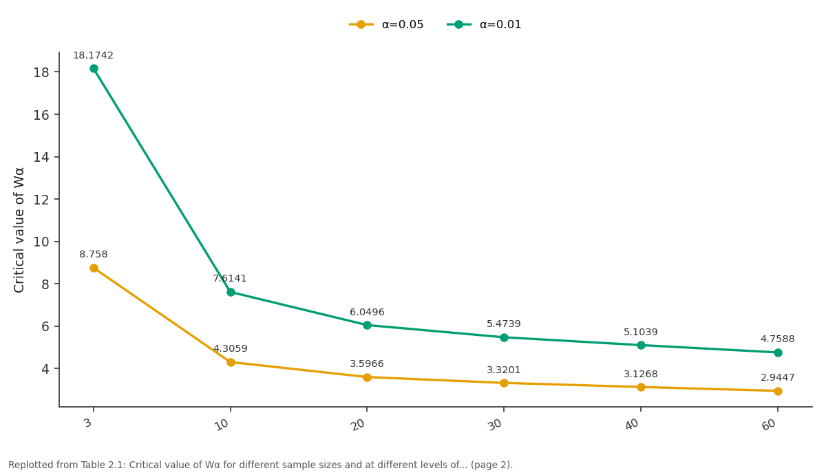
α=0.05 and α=0.01: 3 vs 10 vs 20 vs 30 vs 40
Replotted from Table 2 (page 2) of the original paper. Every bar is the paper's own table value.
View source evidence ↗Figures & tables
From the original paper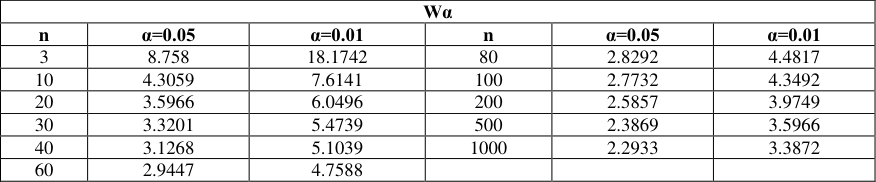 Table 2
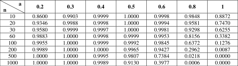 Table 4
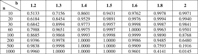 Table 4
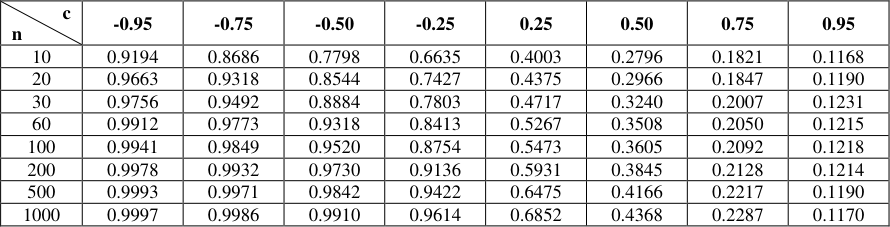 Table 4
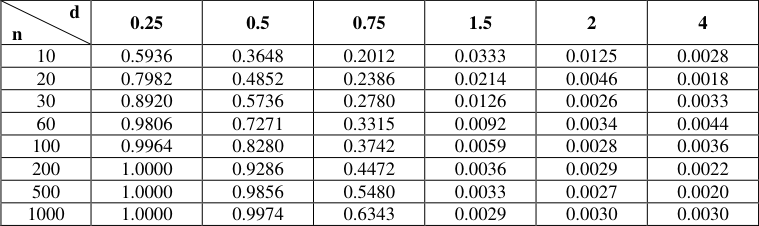 Table 4
Introduction
derived a family of distributions using the method of translation and was called as Johnson family of distributions, which provides flexibility of covering wide varieties of distributional shapes. The advantage of Johnson system of distributions is that it approximates commonly used continuous distributions such as Normal, Log-normal, Gamma, Beta, Exponential distributions. Gerald & Samuel (1967) [4] have shown these distributions as special cases of Johnson system of distributions. Due to its flexible nature, this distribution has wide applications. For example, the S B distribution is used as a model for human exposure data; see Flynn (2004) [2] , Mage (1980) [8] used it for ambient air pollution, Kotteguda (1987) [7] for rainfall distribution, Zang et. al, (2003) [9] for forestry and Konduru et al., (2013) [6] for Infrared brightness temperature distribution of the deep convective clouds. This distribution is also very useful in complicated data set like microarray data analysis, see Florence George (2007) [3] etc. An outlier is defined as an observation that deviates from the rest of the data in some sense. In this paper, a test statistic is developed from a statistic used in the case of a sample from Normal distribution for detection of an upper outlier from Johnson S B distribution when all the parameters are known. For this, Johnson S B distribution is firstly transformed into Standard normal distribution using some suitable transformation. Then the critical region of a test statistic of Normal distribution as given in Barnett and Lewis (1994) [1] is used for obtaining the critical region for Johnson S B distribution.
Johnson SB distribution and test statistic
Let 𝑋 1 , 𝑋 2 , ⋯ , 𝑋 𝑛 be the n observations from Johnson S B distribution and 𝑋 (1) , 𝑋 (2) , ⋯ , 𝑋 (𝑛) be the corresponding order statistics of these n observations. The p.d.f of Johnson S B distribution is given by:
where 𝜉 is the location parameter, 𝜆 is the scale parameter and 𝛿 and 𝛾 are shape parameters. By making a transformation
the density (2.1) transforms to a standard normal distribution i.e.
Let z 1 , z 2 , ⋯ , z n be n observations of normal distribution corresponding to the n observations X 1 , X 2 , ⋯ , X n and z (1) , z (2) , ⋯ , z (n) be the corresponding order statistics of the n transformed observations. The null hypothesis H 0 states that there is no outlying observation in the sample while the alternative hypothesis H 1 states that there is one outlying observation on the right side. The test statistic for detection of a single upper outlier of a sample from a normal distribution with σ 2 known is given in Barnett and Lewis (1994) [1] as
The α level critical region for this statistic is T > T α , where T α is the critical value of T at α level of significance and its tabulated values are given by Barnett and Lewis (1994) [1] for different sample sizes at levels of significance 5 and 1 percent. This test statistic when used for Johnson S B distribution using transformation (2.2) becomes
As the transformation (2.2) is order preserving, z (n) = γ + δ ln (
Let exponential of T be denoted by W, then
Corresponding to the size α critical region T > T α of the statistic T, the critical region of the statistic W is W > W α .
As W is a function of sample values from Johnson S B distribution alone, it can be considered as a suitable test statistic for detection of an upper outlier for the case of Johnson S B distribution. The critical values W α are tabulated in Table 2.1. for 5 and 1 percent significance levels and for different values of n between 3 and 1000. As the derivation of the critical values W α is independent of the parameters(ξ, λ, γ, δ), they can be used for any Johnson S B distribution.
| Wα | — | — | — | — | — |
|---|---|---|---|---|---|
| n | α=0.05 | α=0.01 | n | α=0.05 | α=0.01 |
| 3 | 8.758 | 18.1742 | 80 | 2.8292 | 4.4817 |
| 10 | 4.3059 | 7.6141 | 100 | 2.7732 | 4.3492 |
| 20 | 3.5966 | 6.0496 | 200 | 2.5857 | 3.9749 |
| 30 | 3.3201 | 5.4739 | 500 | 2.3869 | 3.5966 |
| 40 | 3.1268 | 5.1039 | 1000 | 2.2933 | 3.3872 |
| 60 | 2.9447 | 4.7588 |
Table text extracted from the original PDF; superscript letters are shown inline. The original table image is below.
View original table image
Examples
For highlighting the utility of the statistic, the following 20 observations were taken from the Census data of India taken in the year 2011, (in, 000). 1028610, 1045547, 1062388, 1095722, 1112186, 1128521, 1160813, 1176742, 1192506, 1223581, 1238887, 1254019, 1283600, 1298041, 1312240, 1339741, 1352695, 1365302, 1388994, 1399838. This is used in the following examples when the outlying observation is from another sample with a shift in one or all the parameters. The critical value at 5% level of significance for all the examples considered below is 3.5966. Then an outlying observation was introduced by deviating each of the parameters as follows.
Example.3.1: For introducing a contaminant observation with a shifted location parameter, another sample of Johnson S B distribution has to be generated with a location parameter ξ + aλ, where the range of a should be such that 0 < a < 1 for the new observations to lie within the range of the original sample. Here for this example the value of a was taken as 0.5 and a sample with a shifted location parameter was generated. The largest observation of the first sample was replaced with the largest observation of the second sample. Test statistic W U was calculated and was equal to 9.898013 which fall in the critical region at 5% level of significance. Hence, the largest observation of this sample was declared as a contaminant observation.
Example.3.2:
For introducing an outlier with a shift in the scale parameter, another sample of Johnson S B distribution with scale parameter b λ, with b>1, was generated. Here again for the new sample to be within the range of the old one, b should be in the
The largest observation of the first sample was replaced with the largest observation of the second sample. The calculated value of the test statistic W L was equal to 9.152462. On comparison with critical value at 5% level of significance it was found that the calculated value is larger than the critical value. Hence, the null hypothesis gets rejected. This implies that the largest observation is an outlier.
Example.3.3:
For studying the effect of a shift in the shape parameter, another sample with a shift c in shape parameter was generated. To get a sample with finite values, the value of c should be chosen so as to fall in the interval (-(ξ + λ), (ξ + λ)), i.e.
-(ξ + λ) < c < (ξ + λ). In this example, c was taken as 0.5. The largest observation of the first sample was replaced with the largest observation of the second sample. On computation of the test statistic W U it was found to be 3.743415, and thereby the largest observation was declared as a contaminant observation as it was larger than the corresponding critical value.
Example.3.4:
Now for detection of outlying observation arising due to a shift in the shape parameter δ, the second sample was generated with a shift d (where d > 0, for this example d was taken as 0.5) in shape parameter. The largest observation of the first sample was replaced with the largest observation of the second sample. Test statistic W U was calculated and found to be equal to 5.336801. This on comparison with the critical value at 5% level of significance, the null hypothesis gets rejected. This infers that the largest observation to be an outlying observation.
Example. 3.5:
Now for considering the presence of outlier due to a shift in all the four parameters, a second sample was generated with a shift in all the four parameters, i.e. ξ + aλ, bλ, c γ and dδ, where 0 < a < 1,
with a=0.5, b=0.75, c=0.5 and d=0.5 respectively. The largest observation of the first sample was replaced with the second sample. Test statistic W U was calculated and it was equal to 5.820842. This on comparison with critical value was found to be lying in the critical region. This implies that largest observation is a contaminant observation.
Performance study
All the performance studies were done using simulation technique. The performance study was done for slippage alternatives for location, scale and both the shape parameters. For a slippage alternative of the location parameter, a random sample of size n was generated using R software from a Johnson S B distribution with location parameter ξ(=20), scale parameter λ(=10), with two shape parameters γ(=1) and δ(=2) (known). For introducing a contaminant observation another sample of Johnson S B distribution with a shift, (aλ), where 0 < a < 1 in the location parameter was generated. The largest observation of the original sample was replaced with the largest observation of the second sample. The value of the test statistic W U was calculated at 5% level of significance. Simulation study was carried out for sample sizes n = 10(10)30, 60, 100, 200, 500, 1000 and different values of a. Here, the process was simulated 10,000 times and the number of times the test statistic falling in the critical region was noted. The probability of rejection of the null hypothesis is then the ratio of total number of times the null hypothesis was rejected to the total number of trials, i.e. 10,000. These probabilities for different sample sizes-n and different values of a between 0.2 and 1 are shown in the table 4.1. From table 4.1, it can be seen that the performance of the test is reasonably good enough for a shift of aλ in the location parameter with values of a up to 0.5, beyond that it starts declining. This is due to the fact that larger values of the location parameter leading to a smaller value of the statistic W U as observed from (2.5). Also for large values of n, W U being a fraction of two very small quantities tends towards zero with an increase in the value of δ.
| d n | 0.25 | 0.5 | 0.75 | 1.5 | 2 | 4 |
|---|---|---|---|---|---|---|
| 10 | 0.5936 | 0.3648 | 0.2012 | 0.0333 | 0.0125 | 0.0028 |
| 20 | 0.7982 | 0.4852 | 0.2386 | 0.0214 | 0.0046 | 0.0018 |
| 30 | 0.8920 | 0.5736 | 0.2780 | 0.0126 | 0.0026 | 0.0033 |
| 60 | 0.9806 | 0.7271 | 0.3315 | 0.0092 | 0.0034 | 0.0044 |
| 100 | 0.9964 | 0.8280 | 0.3742 | 0.0059 | 0.0028 | 0.0036 |
| 200 | 1.0000 | 0.9286 | 0.4472 | 0.0036 | 0.0029 | 0.0022 |
| 500 | 1.0000 | 0.9856 | 0.5480 | 0.0033 | 0.0027 | 0.0020 |
| 1000 | 1.0000 | 0.9974 | 0.6343 | 0.0029 | 0.0030 | 0.0030 |
Table text extracted from the original PDF; superscript letters are shown inline. The original table image is below.
View original table image
| c n | -0.95 | -0.75 | -0.50 | -0.25 | 0.25 | 0.50 | 0.75 | 0.95 |
|---|---|---|---|---|---|---|---|---|
| 10 | 0.9194 | 0.8686 | 0.7798 | 0.6635 | 0.4003 | 0.2796 | 0.1821 | 0.1168 |
| 20 | 0.9663 | 0.9318 | 0.8544 | 0.7427 | 0.4375 | 0.2966 | 0.1847 | 0.1190 |
| 30 | 0.9756 | 0.9492 | 0.8884 | 0.7803 | 0.4717 | 0.3240 | 0.2007 | 0.1231 |
| 60 | 0.9912 | 0.9773 | 0.9318 | 0.8413 | 0.5267 | 0.3508 | 0.2050 | 0.1215 |
| 100 | 0.9941 | 0.9849 | 0.9520 | 0.8754 | 0.5473 | 0.3605 | 0.2092 | 0.1218 |
| 200 | 0.9978 | 0.9932 | 0.9730 | 0.9136 | 0.5931 | 0.3845 | 0.2128 | 0.1214 |
| 500 | 0.9993 | 0.9971 | 0.9842 | 0.9422 | 0.6475 | 0.4166 | 0.2217 | 0.1190 |
| 1000 | 0.9997 | 0.9986 | 0.9910 | 0.9614 | 0.6852 | 0.4368 | 0.2287 | 0.1170 |
Table text extracted from the original PDF; superscript letters are shown inline. The original table image is below.
View original table image
| b n | 1.2 | 1.3 | 1.4 | 1.5 | 1.6 | 1.8 | 2 |
|---|---|---|---|---|---|---|---|
| 10 | 0.5133 | 0.7156 | 0.8601 | 0.9431 | 0.9762 | 0.9978 | 0.9971 |
| 20 | 0.6184 | 0.8454 | 0.9529 | 0.9891 | 0.9976 | 0.9994 | 0.9940 |
| 30 | 0.6842 | 0.8994 | 0.9773 | 0.9957 | 0.9998 | 0.9987 | 0.9841 |
| 60 | 0.7988 | 0.9651 | 0.9975 | 0.9997 | 1.0000 | 0.9963 | 0.9501 |
| 100 | 0.8685 | 0.9868 | 0.9993 | 0.9998 | 0.9999 | 0.9890 | 0.8768 |
| 200 | 0.9396 | 0.9978 | 1.0000 | 1.0000 | 0.9986 | 0.9485 | 0.6480 |
| 500 | 0.9838 | 0.9998 | 1.0000 | 1.0000 | 0.9909 | 0.7593 | 0.1916 |
| 1000 | 0.9960 | 1.0000 | 1.0000 | 1.0000 | 0.9601 | 0.4141 | 0.0145 |
Table text extracted from the original PDF; superscript letters are shown inline. The original table image is below.
View original table image
| a n | 0.2 | 0.3 | 0.4 | 0.5 | 0.6 | 0.8 | 1 |
|---|---|---|---|---|---|---|---|
| 10 | 0.8600 | 0.9903 | 0.9999 | 1.0000 | 0.9998 | 0.9848 | 0.8872 |
| 20 | 0.9346 | 0.9988 | 0.9998 | 1.0000 | 0.9994 | 0.9581 | 0.7470 |
| 30 | 0.9580 | 0.9999 | 0.9997 | 1.0000 | 0.9981 | 0.9298 | 0.6255 |
| 60 | 0.9883 | 1.0000 | 0.9998 | 0.9999 | 0.9953 | 0.8156 | 0.3382 |
| 100 | 0.9955 | 1.0000 | 0.9999 | 0.9992 | 0.9845 | 0.6372 | 0.1276 |
| 200 | 0.9989 | 1.0000 | 1.0000 | 0.9965 | 0.9427 | 0.2962 | 0.0087 |
| 500 | 1.0000 | 1.0000 | 0.9995 | 0.9807 | 0.7384 | 0.0218 | 0.0000 |
| 1000 | 1.0000 | 1.0000 | 0.9989 | 0.9130 | 0.3977 | 0.0006 | 0.0000 |
Table text extracted from the original PDF; superscript letters are shown inline. The original table image is below.
View original table image
Proceeding in a similar manner, for a slippage alternative of the scale parameter, a sample was generated and for introducing an outlying observation, another sample was generated with a shift b, where ξ λ ⁄ < b < 1+ ξ λ ⁄ in the scale parameter. The largest observation of the first sample was replaced with that of the second sample. The value of the test statistic W U was calculated at 5% level of significance. This process was repeated 10,000 times and in this process, the number of times the null hypothesis was rejected was observed. The probabilities of rejection of null hypothesis for sample sizes n = 10(10)30, 60, 100, 200, 500, 1000 and for different value of b between 1.2 and 2 are shown in the table 4.2. It can be observed from this table, that for negative values of shift, the test statistic certainly identifies the contaminant observation, whereas for positive values of shift the performance of test statistic is extremely poor. For c=0 the performance is very good even for small sample sizes. Now, for a slippage alternative of the shape parameter (δ), a sample was generated and for introducing a contaminant observation, another sample with a shift d in the shape parameter was generated. The largest observation of the first sample was replaced with the corresponding observation of the second sample and a new sample was formed. Then the test statistic W U was calculated at 5% level of significance. This process was repeated 10,000 times for different sample sizes and for different values of d and the probability of identification of the contaminant observation was obtained. These probabilities for sample sizes n = 10(10)30, 60, 100, 200, 500, 1000 and for different values of d between 0.25 and 4 are shown in table 4.4.
References
9 in the original paper- Barnett V, Lewis T. Outliers in Statistical Data. John Wiley, 1994.
- Flynn MR. The 4 parameter lognormal (S B ) model of human exposure. Ann Occup Hyg. 2004; 48:617-22.
- George F. Johnson's system of distribution and Microarray data analysis. Graduate Theses and Dissertations, University of South Florida, 2007.
- Hahn J Gerald, Shapiro S Samuel. Statistical model in Engineering, John Wiley and sons, 1967.
- Johnson NL. Systems of frequency curves generated by methods of translation. Biometrica. 1949; 58:547-558.
- Konduru RT, Kishtawal CM, Shah S. A new perspective on the infrared brightness temprative distribution of the deep convective clouds. Springer, 2013.
- Kottegoda NT. Fitting Johnson S B curve by method of maximum likelihood to annual maximum daily rainfalls. Water Resour Res. 1987; 23:728-732.
- Mage DT. An explicit solution for S B parameters using four percentile points, Technometrics. 1980; 22:247-251.
- Zhang L, Packard PC, Liu C. A comparison of estimation methods for fitting Weibull and Johnson's S B distributions to mixed spruce-fir stands in northeastern North America. Can J Forest Res. 2003; 33:1340-1347.