
Research article · 2018 · Full text
International Journal of Statistics and Applied MathematicsOn skew generalized extreme value-ARMA model: An application to average monthly temperature (1901-2016) in Nigeria
Volume 3(5) · Pages 20–27
Research areasEnergy Load and Power Forecasting
Abstract
Author-writtenThis study describes the approach for modeling extreme and lengthy time-varying series of an Autoregressive Moving Average of order ( , ) p q via a Skew Generalized Extreme Value distribution as the white noise. This approach establishes the procedure for parameters’ estimation and their standard errors for the SGEV-ARMA ( , ) p q model via the iterative Fisher information scores derived from the Maximum Likelihood Estimation for a chosen optimal degree of flexibility (bandwidth)" " . The study was applied to a lengthy series of average monthly temperature (report in oC) of Lagos, Nigeria from January 1901 to December 2016 with 1381 data points. It was noted that SGEV-ARMA (3,3) recorded a subjacent model performance error via the evaluated indexes of AIC, BIC and HQIC (103.02, 141.35 & 124.50) respectively compare to an intensive error performance in the white noise Gaussian-ARMA (3, 3) with (108, 144.4 & 129.26) respectively. In addition, the forecast error indexes with the SGEV subjected white noise were miniaturized compared to the Gaussian white noise.
Summary
Source-checkedPlain-language reading of the full paper, prepared with AI and checked against the text. Each point links to the authors' own words.
Why it matters
- Extreme value theory is a critical tool for modeling phenomena across various fields, including meteorology and risk management. View evidence ↗
- Accurate estimates of extreme events, such as precipitation, are essential for planning infrastructure like dams and managing flood frequency. View evidence ↗
The question
- The study aims to use the Skew Generalized Extreme Value (SGEV) distribution as the stochastic error distribution within an Autoregressive Moving Average (ARMA) model to handle time-varying trends. View evidence ↗
What they did
- The researchers analyzed 1,381 data points of average monthly temperature in degrees Celsius from Lagos, Nigeria, spanning from January 1901 to December 2016. View evidence ↗
- Based on the analysis of the weather series, the optimal order for the ARMA model was determined to be (3, 3). View evidence ↗
What they found
- Stationarity tests (ADF, PP, and KPSS) with p-values of 0.01, 0.01, and 0.0382 respectively indicated a high probability that the temperature data is stationary. View evidence ↗
- The temperature data showed evidence of extreme values, likely lower outliers, as indicated by a skewness value of 3.3803. View evidence ↗
- The SGEV-ARMA (3,3) model outperformed the Gaussian-ARMA (3,3) model, showing lower AIC (103.02 vs 108), BIC (141.35 vs 144.4), and HQIC (124.50 vs 129.26). View evidence ↗
What it means
- The authors conclude that the SGEV white-noise approach provides superior model performance and better handles skewness and kurtosis compared to the conventional Gaussian error term in ARMA models. View evidence ↗
Visual summary
1 visualsIllustrations explain the paper; they do not show study data.
Model Comparison Concept
AI-generated conceptual illustration (Average monthly temperature time-series data in Nigeria). It explains the idea and does not show study data.
View source evidence ↗Figures & tables
From the original paper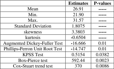 Table 1
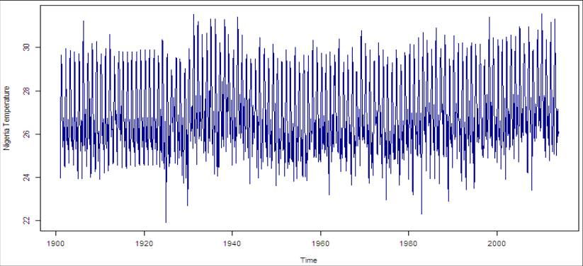 Figure 1
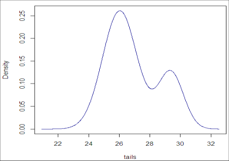 Figure 2
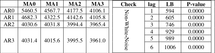 Table 2
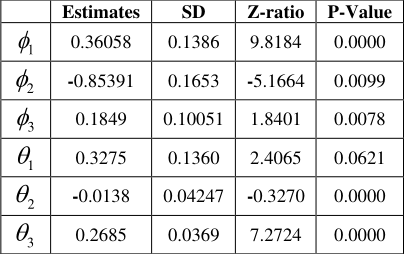 Table 3
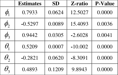 Table 3
Introduction
The origin of extreme value theory started its course by Gnedenko (1943) [10] when it was used to study the maxima series of Gaussian subjected variables under general hypothesis of limiting distribution called Generalized Extreme Value (GEV) distribution for series of extreme (s), lengthy series, lengthy observations, ecological observations, climate observations etc. Its course was extended when an unusual or usual event takes place regardless of whether or not it is catastrophic or when an event causes catastrophes (Farago and Katz, 1990 [6] ; Faranda et al. 2012 [7] .). However, its development could be traced back to the work done by Bernoulli in 1975 [3] . Kotz and Nadarajah (2000) [11] and its first application was made by Fuller in 1914 [8] . It is based on large deviations from the median of probability distributions such that the theory assesses the type of probability distribution generated by processes. Rieders (2014) [17] affirmed that limiting distributions (which are distinct from the normal distribution) are the Extreme Value Distributions (EVD) for maximum, minimum or extreme lengthy contaminated series or collection of observations of either dependent or covariates random variable (s). It is widely used in modeling phenomena in disciplines, such as structural hydrology, meteorology, engineering, finance, earth sciences, traffic prediction and risk management. Estimates of extreme precipitation are consistent in forecasting planning infrastructures such as dams flood frequency etc. Engineers often need such statistics for the design of structures for flood protection using Areal Reduction Factors (ARFs) to convert quantiles for point rainfall to the corresponding quantiles of areal rainfall. ARFs have been derived empirically by estimating the areal rainfall as a function of point rainfall measurements e.g. Natural Environment Research Council (NERC) (1975) [13] ; Bell (1976) [2] ; or by statistical modeling (Bacchi and Ranzi, 1996) [1] .
Three approaches had been in existence for the practical applications extreme value-the first method evolves deriving block maxima (that is maxima/minima) series as a preliminary step. The approach relies partly on the results of the Fisher-Tippett-Gnedenko theorem, leading to the Generalized Extreme Value Distribution (GEVD) being selected for fitting. The second method relies on extracting "Peak over Threshold" (POT) that is peak values above or below a certain threshold from a continuous record while the third approach tries to strike the balance between the block maxima and peak over threshold approaches via r th -largest order statistics approach (Ragulina and Reitan, 2017) [16] . Chavez-Demoulin and Davison (2012) [5] superposed monthly maximum river flow at the station Muota-Ingenbohl in Switzerland, for the years 1923-2008 by fitting a nonparametric GEV with time dependent location parameter where "" plays the same role as the bandwidth in local likelihood estimation to the random effects model. In addition, Laurini & Pauli (2009) [12] , applied it using Bayesian computational tools. Ning and Bloomfield (2017) [4] water flow dataset is collected from French Broad River at Asheville in North Carolina. The datasets contain annual maximum water flow level from 1941 to 2009 and used the Dependent Generalized Extreme Value (DGEV) model as the white noise of the Autoregressive model to explain the water flow phenomena. Hence, this article subjected the Skew Generalized Extreme Value (SGEV) distribution as the stochastic error distribution of Autoregressive Moving Average (ARMA) as a deterministic time varying model for trend or non-trend effect and used the iterative Fisher information scores via the maximum likelihood method of estimation in estimating their standard errors for a chosen optima degree of flexibility (bandwidth) "" .
Specification of the skew generalized extreme value-autoregressive moving average (SGEV-ARMA)
A stochastic process of t y is said to follow an Autoregressive Moving Average (ARMA) of order ( , )
Where, is the Gamma function with identity
That is, SGEV-ARMA ( , ) pq . Ribereau et al. (2011) [15] defined the Probability Density Function (PDF) of a random variable () t y for Skew Generalized Extreme Value (SGEV) distribution to be ( ) ( 1) ( ) ( )
Gy are the PDF and Cumulative Distribution Function (CDF) of the Generalized Extreme Value (GEV) distribution respectively, where must be strictly greater than -1.
Parameter Estimation
The Hessian matrix of the parameter space, 2
Such that the () H is a block diagonal matrix and a square matrix of n by n dimension depending on the order of the SGEVARMA, that is the order of ( , ) pq .
The Fisher Scoring algorithm, S are the Fisher information and Score matrixes respectively to be evaluated by via Newton-Raphson iterative procedure for a chosen value of the degree of flexibility measures () that must be strictly greater than one.
Model identification criteria
Model selection via information criteria is being defined as
However, Tsay (2016) [18] defined the information criteria in terms of the Akaike's Information Criteria (AIC), Bayesian's Information Criteria (BIC) and Hannan and Quinn Information Criteria (HQIC). The criteria defined will be extended to by substituting the maximum likelihood of the SGEV-ARMA to the residual variance needed.
Analysis and discussion of results
The average monthly series of temperature of Lagos, Nigeria from January 1901 to December 2016 was used. Observations are reported in Degree Celsius ( o C), recorded on monthly bases starting from the inception of meteorological section under the ministry of environment. The models' estimation and Exploratory Data Analysis utilized One thousand three hundred and eighty one (1381) data points of the average monthly temperature. All the data points maintained the same unit of measurement of o C. The kernel density plot confirmed the unusual emerged of the fat-tailed of the frequency distribution of the weather report meteorological distributed. It is nothing but merged mesokurtic distributions. (3, 3) in terms of parameterization and indexes. Firstly, is to be noted that the no differencing in any form was subjected to the series, since it was stationary at raw. The crucial step in an appropriate model performance is the determination of optimal model via the models with subjacent performance criteria; the AIC, BIC and HQIC for the Gaussian white-noise were (108, 144.4 and 129.26) respectively at optima selected of (3, 3) compared to SGEV white-noise with lesser AIC, BIC and HQIC (103.02, 141.35, 124.50) respectively, that best described and captured lesser stochastic error. In addition, the mean of the two models differs by 0.906, connoting a smaller magnitude in each of the models' clustering around the mean o C, but the variation (1.8075) in the SGEV-ARMA (3, 3) model was dinky compared to the Gaussian-ARMA (3, 3). Furthermore, the evaluation of the computed forecast error indexes of the two models of the weather series report were estimated. ). The error forecast of the SGEV-ARMA is subjacent to Gaussian-ARMA, suggesting a more robust evaluation and performance of the incorporated non-white-noise of the SGEV.
Preliminary and descriptive analysis
Preliminary and descriptive analysis
Model estimation and analysis
Model estimation and analysis
Conclusions
In conclusion, the recorded weather report series in o Cs maintained a near steady and constant trend around the 90 to 100 percentiles of the range and minimum o C was recorded within the first quarter of the year 1920 with the trend around 10 to 20 percentiles not really steady and constant. The series was favored with a miniaturized chance of 0.01 of non-stationary. In addition, the variation absolution via skewness and kurtosis; and model performance was superincumbent in the SGEV whitenoise compression in matchmaking with the conventional Gaussian error term subjected to the ARMA.
Figures and tables from the paper
| — | Estimates | P-values |
|---|---|---|
| Mean | 26.91 | ----- |
| Min. | 21.90 | ----- |
| Max. | 31.57 | ----- |
| Standard Deviation | 1.8075 | ----- |
| skewness | 3.3803 | ----- |
| kurtosis | -0.6504 | ----- |
| Augmented Dickey-Fuller Test | -16.666 | 0.01 |
| Phillips-Perron Unit Root Test | -14.747 | 0.01 |
| KPSS Test | 0.5154 | 0.0382 |
| Box-Pierce test | 592.44 | 0.0023 |
| Cox-Stuart trend test | 370 | 0.0086 |
Table text extracted from the original PDF; superscript letters are shown inline. The original table image is below.
View original table image
| — | MA0 | MA1 | MA2 | MA3 | — | Check | lag | LB | P-value | — |
|---|---|---|---|---|---|---|---|---|---|---|
| AR0 | 5460.5 | 4567.7 | 4177.5 | 4106.1 | Non-White-Noise | 1 | 594 | 0.0000 | ||
| AR1 | 4682.3 | 4322.5 | 4142.6 | 4105.8 | 2 | 605 | 0.0000 | |||
| AR2 | 4030.6 | 4031.8 | 3994.4 | 3965.4 | 3 | 746 | 0.0000 | |||
| AR3 | 4031.4 | 4015.6 | 3995.5 | 3961.0 | 4 | 929 | 0.0000 | |||
| 5 | 989 | 0.0000 | ||||||||
| 6 | 1006 | 0.0000 |
Table text extracted from the original PDF; superscript letters are shown inline. The original table image is below.
View original table image
References
18 in the original paper- Bacchi B, Ranzi R. On the derivation of the areal reduction factor of storms. Atmospheric Research. 1996; 42:123-135.
- Bell FC. The areal reduction factors in rainfall frequency estimation. Institute of Hydrology, Wallingford, 1976, 35.
- Bernoulli N. De Usu Artis conjectandi in lure. Doctoral Thesis, Basel. In: Die Werke von Jakob Bernoulli. 1975; 3(1):287326.
- Ning B, Bloomfield P. Bayesian inference for generalized extreme value distribution with Gaussian copula dependence. Cornell University Library 2017. ArXiv: 1703.00968v1 [stat. ME].
- Chavez-Demoulin V, Davison AC. Modeling Time Series Extremes. REVSTAT-Statistical Journal, 2012; 10(1):109-133.
- Faragó T, Katz RW. Extremes and design values in climatology. World Meteorological Organization WMO-TD. 1990; 386(14):46.
- Faranda D, Lucarini V, Turchetti G, Vaienti S. Generalized extreme value distribution parameters as dynamical indicators of stability. International Journal of Bifurcation and Chaos. 2012; 22(11):1793-6551. doi.org/10.1142/S0218127412502768.
- Fuller WE. Flood flows. ASCE Trans. 1914; 77:567-617.
- Galina R, Trond R. Generalized extreme value shape parameter and its nature for extreme precipitation using long time series and the Bayesian approach. Hydrological Sciences Journal, 2017; 62(6):863-879. doi:10.1080/02626667.2016.1260134. 2150-3435.
- Gnedenko B. Sur la distribution limite du terme maximum d'une série aléatoire. The Annals of Mathematics. 1943; 44:423453. https://www.jstor.org/stable/1968974
- Kotz S, Nadarajah S. Extreme Value Distributions: Theory and Applications. London: Imperial College Press, 2000.
- Laurini F, Pauli F. Smoothing sample extremes: The mixed model approach. Computational Statistics and Data Analysis. 2009; 53:3842-3854.
- Natural Environment Research Council (NERC). Flood studies report. NERC, London, 1975:2.
- Padoan SA, Wand MP. Mixed model-based additive models for sample extremes. Statistical Probability Letter. 2008; 78:2850-2858.
- Ribereau P, Masiello E, Naveau P. Skew generalized extreme value distribution: probability weighted moments estimation and application to block maxima procedure. Communication in Statistics-Theory and Methods, Taylor & Francis, 2014, 1-25. https://hal.archives-ouvertes.fr/hal-01018877
- Ragulina G, Reitan T. Generalized extreme value shape parameter and its nature for extreme precipitation using long time series and the Bayesian approach. Hydrological Sciences Journal, 2017; 4(1):2150-3435. doi: 10.1080/02626667.2016.1260134.
- Rieder HE. Extreme Value Theory: A primer. Lamont-Doherty Earth Observatory, 2014.
- Tsay RS. Lecture Notes of Bus 41202 (Spring) Analysis of Financial Time Series, 2016.
Cited by 1
From OpenAlex, OpenCitations and reference lists read by Scinovex
- Parametric Poisson Bifurcated Autoregressive Process: Application to Worldwide, Regional, and Peculiar Countries’ of Automobile Production ↗
Rasaki Olawale Olanrewaju, Sodiq Adejare Olanrewaju, Toyin Omoyeni Oguntola, Wasiu Adesoji Adepoju · Journal of Mathematical Analysis and Modeling · 2023
This article introduces Bifurcated Autoregressive (BAR) process with two apart marginal distribution error terms of w2 and w2+1 of Poisson white noises to make it Poisson Bifurcated Autoregressive (PBAR) in a parametric setting. The statistical definition of PBAR (1) process with parameters B1 and B2 that must be |B1 | and |B2 |<1 for stationary process was spelt-out. Weighted Least…
❝ 0PDF