
Research article · 2018 · Full text
International Journal of Statistics and Applied MathematicsDetermination of variable sampling plans based on weighted expansion factor for a non-normal lomax process
Volume 3(2) · Pages 170–177
Research areasAdvanced Statistical Process MonitoringAdvanced Statistical Methods and ModelsScientific Measurement and Uncertainty Evaluation
Abstract
Author-writtenThis article deals with designing procedure of Lomax variable sampling plans by utilizing weighted factor for a heavy tailed non-normal family. Variable sampling plans are preferred because of its efficiency in sample size and also used when the nature of the quality characteristic is measurable. If the underlying distribution is non-normal then the standard normal procedures could not be used. In many industrial situations, the quality characteristics does not follow a normal or Gaussian pattern. Hence to develop new sampling plans, an attempt has been made by assuming a heavy tailed Lomax distribution. The selection of variable sampling plans based on AQL, LQL and minimum tangent angle technique using Lomax distribution has been designed using weighted factor method. Tables are constructed and illustration is given for easy selection of sampling plans.
Summary
Source-checkedPlain-language reading of the full paper, prepared with AI and checked against the text. Each point links to the authors' own words.
Why it matters
- Variable sampling plans are advantageous because they are more efficient in terms of sample size when quality characteristics can be measured. View evidence ↗
- Standard normal procedures for sampling are unsuitable for many industrial situations where quality characteristics follow non-normal distributions. View evidence ↗
- The Lomax distribution, also known as the Pareto distribution of the second kind, is a heavy-tailed distribution typically used for reliability estimation and life testing. View evidence ↗
The question
- The authors aim to design new variable sampling plans for non-normal processes by applying a weighted factor method to the heavy-tailed Lomax distribution, indexed by AQL, LQL, and a minimum tangent angle technique. View evidence ↗
What they did
- The sampling plans are developed using an expansion factor that is calculated based on the skewness and kurtosis of the underlying distribution. View evidence ↗
- The authors constructed reference tables to facilitate the easy selection of appropriate sampling plans. View evidence ↗
- The minimum angle method determines the best sampling plan by calculating the tangent of the angle between points representing the Acceptable Quality Level (AQL) and the Limiting Quality Level (LQL). View evidence ↗
What they found
- When U is specified for p1=0.02 and p2=0.06, the plan (105, 2.2877) yields a minimum tangent angle of θ=1.1040. View evidence ↗
- When L is specified for p1=0.02 and p2=0.06, the plan (38, 2.2877) yields a minimum tangent angle of θ=14.7600. View evidence ↗
What it means
- The authors conclude that the minimum angle approach simultaneously minimizes risks for both producers and consumers. View evidence ↗
- The authors suggest that this method of using the minimum tangent angle can be extended to any non-normal distribution. View evidence ↗
Visual summary
2 visualsIllustrations explain the paper; charts are replotted from the paper's own table values.
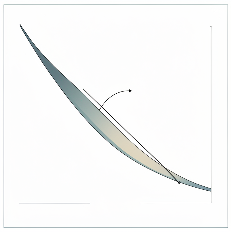
Minimum Tangent Angle Concept
AI-generated conceptual illustration (A mathematical coordinate plane with a curved line). It explains the idea and does not show study data.
View source evidence ↗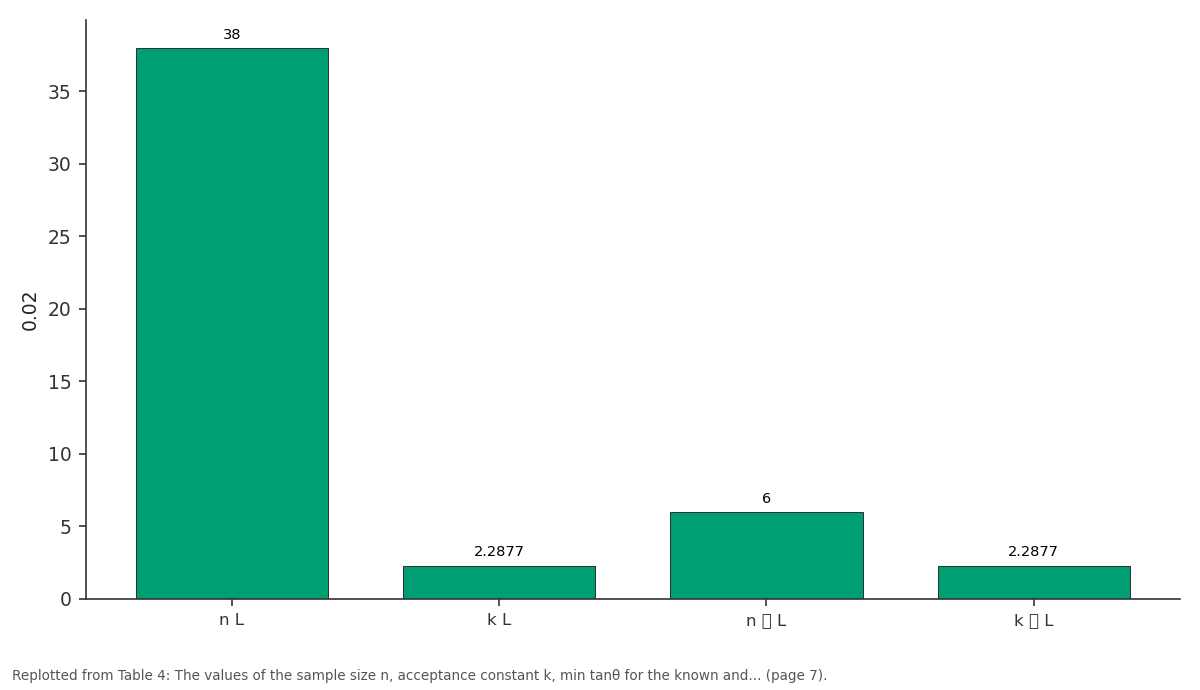
0.02: n L vs k L vs n L vs k L
Replotted from Table 4 (page 7) of the original paper. Every bar is the paper's own table value.
View source evidence ↗Figures & tables
From the original paper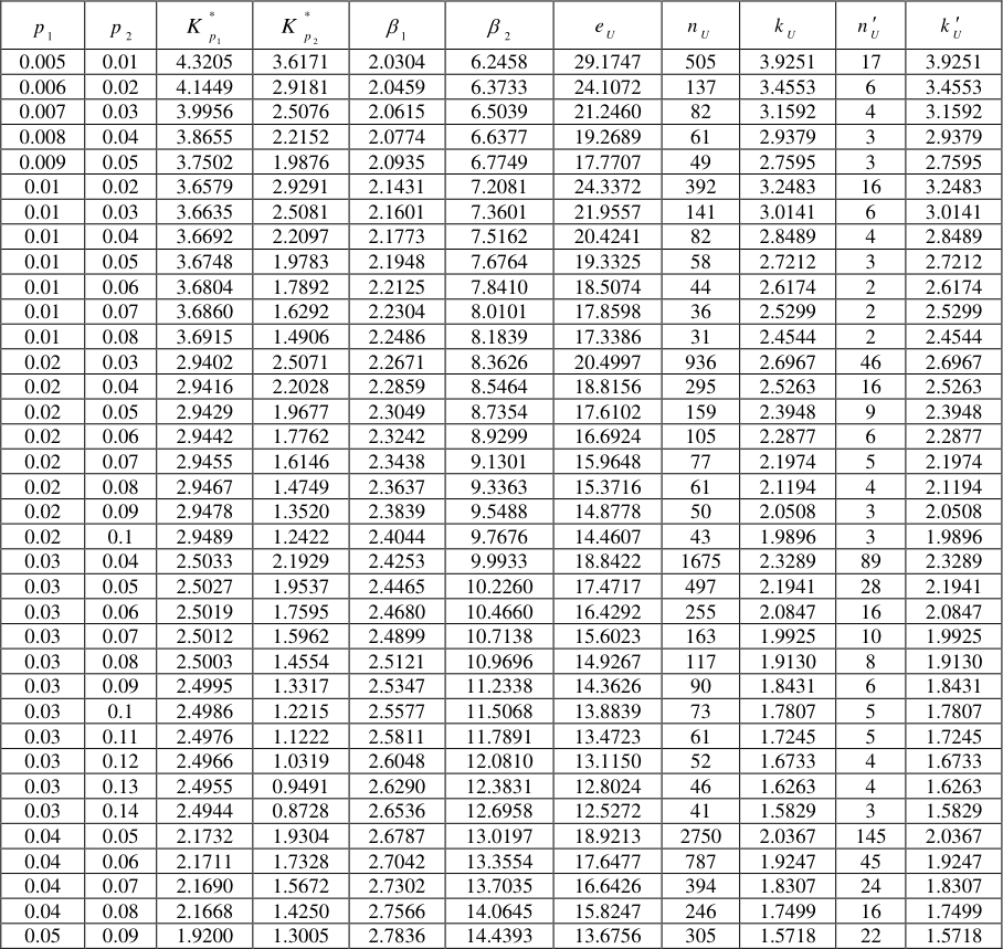 Table 1
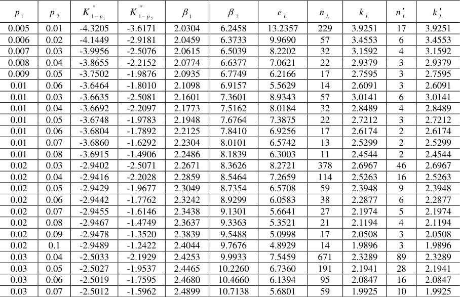 Table 2
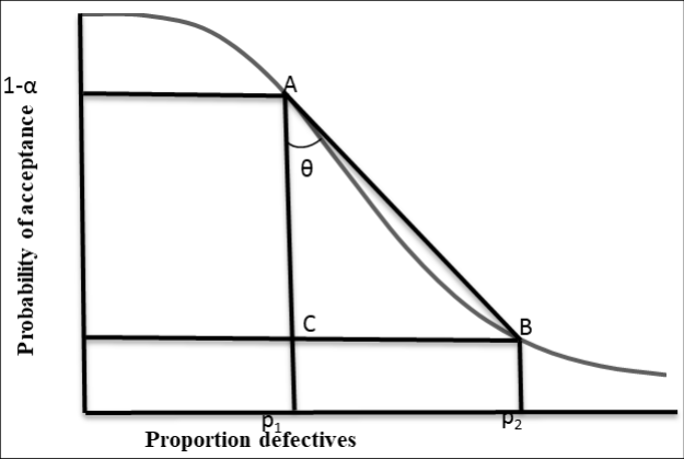 Figure 1
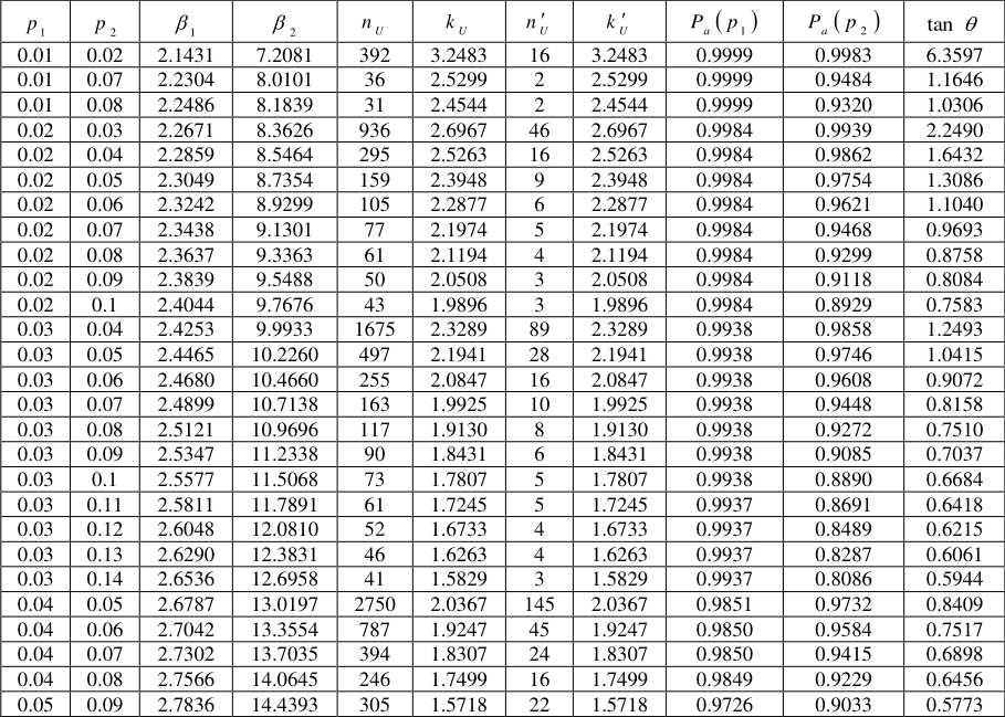 Table 3
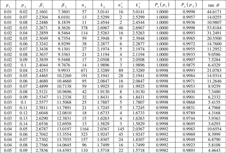 Table 4
Introduction
Even though variable sampling plans have wide range of advantages in sampling plan literature, the main aspect to be considered while employing variable sampling plans is that the distribution of the quality characteristic must be known. In many quality contro sections mostly the underlying distribution of the quality characteristic is assumed to be normal. But in industries there may be a chance for the distribution to be non-normal. It is always not possible to determine the parameters when the process is non-normal. However the procedure for non normal processes has been suggested by authors like, Zimmer and Burr [1] , Owen [2] and Takagi [3] . In this paper a heavy tailed distribution namely Lomax distribution is used to determine the parameters of the sampling plans. It is a special case of generalised Pareto distribution. A Lomax distribution is also called as pareto distribution of second kind is a heavy tailed probability distribution used in life testing and reliability estimation. A heavy tailed distribution generally has a positive and huge kurtosis. Taking advantage of skewness and kurtosis, in this article sampling plans are determined. In this article another approach to determine the sampling plans is by using minimum tangent angle. The smaller the value of the tan θ, closer is the angle θ approaches zero, and the chord length AB in Figure .1 approaches to AC and the ideal condition is reached. It can be understood that whenever the angle is minimised, then the abstract OC curve tends to ideal OC curve. Hence by using this advantage Lomax VSP are developed using minimum angle technique. Devaarul and Jemmy Joyce [4] have developed reliability sampling plans based on minimum angle technique. Soundararajan & Christina [5] have developed single sampling variables plans based on the minimum angle. Bush et.al [6] have considered two points on the Operating Characteristic curve as (AQL, 1-α) and (IQL, 0.5) for minimizing consumer's risk. Bander Al-Zahrani and Mashail Al-Harbi [7] considered the estimation problem of the probability S = P(Y < X) for Lomax distribution based on general progressive censored data. Artur J. Lemonte and Gauss M. Cordeiro [8] proposed a new five-parameter continuous distribution, called McDonald Lomax distribution that extends the Lomax distribution and some other distributions.
Geetha and Vijayaraghavan [9] developed a procedure for determining the parameters of a certain plan to protect both consumer and producer. Wolfgang [10] discussed variable sampling plans based on generalised Pareto distribution. Montgomery [11] observed the effect of normality in variable sampling plans and the methods to detect normality. Jemmy Joyce, Devaarul and Rebecca Edna [12] proposed mixed sampling plans based on the tangent angle, AQL and LQL. Lomax [13] has introduced this distribution in the analysis of business failure data. For any quality characteristic there exists an upper specification limit or lower specification limit or both for determination of parameters. Hence variable sampling plans based on upper and lower specification limits have been developed. Also the parameters for known standard deviation and unknown standard deviation are developed. Variable sampling plans for non normal process had been developed based on the procedure given by Takagi [3] . For any non normal process the skewness and kurtosis plays a vital role. Hence these plans were developed by using the expansion factor which is a function of skewness and kurtosis of the underlying distribution.
Formulation of the sampling plans
A random variable, 'X' is said to follow the Lomax distribution, if the probability density function (pdf) of t is as follows:
The cumulative distribution function (cdf) of Lomax distribution is given by,
where λ is the scale parameter and α is the shape parameter.
Determination of Parameters
are asymptotically normally distributed with the means
Where β1 and β2 represent the skewness and kurtosis of the underlying distribution. The underlying distribution is a Lomax distribution where λ is the scale parameter and α is the shape parameter.
Mean of the Lomax distribution
Mean of the Lomax distribution
Variance of the Lomax distribution
Variance of the Lomax distribution
Skewness of the Lomax distribution
Skewness of the Lomax distribution
Kurtosis of the Lomax distribution
Step 4: Find the expansion factor eU which is a function of β1 and β2.
Step 5: If U is specified determine the corresponding expansion factor eU using the formula:
Step 6: If L is specified determine the corresponding expansion factor eL using the formula:
Algorithm for selection of variable sampling plans when U is specified
Step 1: The scale parameter λ and shape parameter α of Lomax distribution are determined using past experience in the production process.
Step 2: Draw a random sample of n items say x1, x2, x3 …..xn from a lot of size N.
Step 3: Determine the Skewness (β1) and Kurtosis (β2) from the observed data.
Step 4: Now obtain the corresponding mean x and standard deviation σ.
, accept the lot or otherwise reject it. (when σ is known).
Step 6: In case of unknown σ, if
, accept the lot or otherwise reject it.
Designing procedure of the variable sampling plans using the expansion factor (U specified)
The OC function for unknown-sigma plan for a situation when U is specified is
The nU and kU values for unkown sigma plans are
Where Kα and Kβ are the standardised deviates exceeded with the probabilities α and β respectively.
The n and k values for known sigma plans are
Algorithm for selection of variable sampling plans when L is specified
Step 1: The scale parameter λ and shape parameter α of Lomax distribution are determined using past experience in the production process.
Step 2: Draw a random sample of n items say x1, x2, x3 …..xn from a lot of size N.
Step 3: Determine the Skewness (β1) and Kurtosis (β2) from the observed data.
Step 4: Now obtain the corresponding mean x and standard deviation σ.
, accept the lot or otherwise reject it. (When σ is known).
Step 6: In case of unknown σ, if
, accept the lot or otherwise reject it.
Designing procedure of the variable sampling plans using the expansion factor (L specified)
In a similar way when L is specified the OC function for unknown-sigma plan is
The nL and kL values for unkown sigma plans are
Where Kα and Kβ are the standardised deviates exceeded with the probabilities α and β respectively.
The n and k values for known sigma plans are
Construction of tables Table 1 (i)
The values of p1 and p2 are chosen at fixed intervals.
(ii) When U is specified the corresponding values of The values of nU and kU for unknown sigma plans are obtained using equations 14 & 15.
(iv) Similarly the u n and u k values of known sigma plans are obtained using equation 16.
Table 2 (i)
The values of p1 and p2 are chosen.
(ii) When L is the corresponding values of The probability of acceptance are obtained using equation 11 for the values of p1 and p2. (iii)
The corresponding mininimum tangent angle is calculated using equation 23. The probability of acceptance are obtained using equation 17 for the values of p1 and p2. (iii)
The corresponding mininimum tangent angle is calculated using equation 23.
Designing Procedure by Minimum Angle Method
Whenever the angle is minimized, then the abstract OC curve tends to ideal OC curve which leads to best sampling plans. Generally a portion of the abstract OC curve is compared with the ideal OC curve in minimum angle technique. The approach of minimum angle method by considering the tangent of the angle between the lines joining the points (AQL, 1-α) & (LQL, β) is shown in Figure 1.
Thus when the two points on the OC curve such as AQL and LQL are known, the minimum values of the angle tanθ could be calculated. This minimum angle provides a better sampling plan with good discriminating power. It minimizes the angle between the abstract and ideal OC cuves. For a minimum tanθ, the angle θ approaches to zero as the chord AB approaches to AC, hence the ideal condition is reached. This approach minimizes both producers and consumers risk simultaneously. Thus both are benefitted by choosing these plans. The minimum angle method of Lomax variable sampling plans are presented in Table 3 and Table 4. The parameters of Lomax variable sampling plans are chosen from Table 3 and Table 4 corresponding to the minimum angle.
| p 1 | p 2 | 1 | 2 | n L | k L | n L | k L | P p a 1 | P p a 2 | tan |
|---|---|---|---|---|---|---|---|---|---|---|
| 0.01 | 0.02 | 2.1601 | 7.3601 | 57 | 3.0141 | 16 | 3.0141 | 1.0000 | 0.9998 | 44.6171 |
| 0.01 | 0.07 | 2.2304 | 8.0101 | 13 | 2.5299 | 2 | 2.5299 | 1.0000 | 0.9957 | 14.0255 |
| 0.01 | 0.08 | 2.2486 | 8.1839 | 11 | 2.4544 | 2 | 2.4544 | 1.0000 | 0.9936 | 10.9807 |
| 0.02 | 0.03 | 2.2671 | 8.3626 | 378 | 2.6967 | 46 | 2.6967 | 1.0000 | 0.9998 | 53.8184 |
| 0.02 | 0.04 | 2.2859 | 8.5464 | 114 | 2.5263 | 16 | 2.5263 | 1.0000 | 0.9993 | 31.2491 |
| 0.02 | 0.05 | 2.3049 | 8.7354 | 59 | 2.3948 | 9 | 2.3948 | 1.0000 | 0.9985 | 20.5500 |
| 0.02 | 0.06 | 2.3242 | 8.9299 | 38 | 2.2877 | 6 | 2.2877 | 1.0000 | 0.9972 | 14.7600 |
| 0.02 | 0.07 | 2.3438 | 9.1301 | 27 | 2.1974 | 5 | 2.1974 | 1.0000 | 0.9955 | 11.2952 |
| 0.02 | 0.08 | 2.3637 | 9.3363 | 21 | 2.1194 | 4 | 2.1194 | 1.0000 | 0.9933 | 9.0586 |
| 0.02 | 0.09 | 2.3839 | 9.5488 | 17 | 2.0508 | 3 | 2.0508 | 1.0000 | 0.9907 | 7.5284 |
| 0.02 | 0.1 | 2.4044 | 9.7676 | 14 | 1.9896 | 3 | 1.9896 | 1.0000 | 0.9875 | 6.4329 |
| 0.03 | 0.04 | 2.4253 | 9.9933 | 671 | 2.3289 | 89 | 2.3289 | 0.9998 | 0.9993 | 21.0783 |
| 0.03 | 0.05 | 2.4465 | 10.2260 | 191 | 2.1941 | 28 | 2.1941 | 0.9998 | 0.9984 | 14.9314 |
| 0.03 | 0.06 | 2.4680 | 10.4660 | 95 | 2.0847 | 16 | 2.0847 | 0.9998 | 0.9971 | 11.2646 |
| 0.03 | 0.07 | 2.4899 | 10.7138 | 59 | 1.9925 | 10 | 1.9925 | 0.9998 | 0.9953 | 8.9259 |
| 0.03 | 0.08 | 2.5121 | 10.9696 | 42 | 1.9130 | 8 | 1.9130 | 0.9998 | 0.9930 | 7.3480 |
| 0.03 | 0.09 | 2.5347 | 11.2338 | 32 | 1.8431 | 6 | 1.8431 | 0.9998 | 0.9901 | 6.2332 |
| 0.03 | 0.1 | 2.5577 | 11.5068 | 25 | 1.7807 | 5 | 1.7807 | 0.9998 | 0.9868 | 5.4155 |
| 0.03 | 0.11 | 2.5811 | 11.7891 | 21 | 1.7245 | 5 | 1.7245 | 0.9998 | 0.9831 | 4.7968 |
| 0.03 | 0.12 | 2.6048 | 12.0810 | 18 | 1.6733 | 4 | 1.6733 | 0.9998 | 0.9789 | 4.3168 |
| 0.03 | 0.13 | 2.6290 | 12.3831 | 15 | 1.6263 | 4 | 1.6263 | 0.9998 | 0.9744 | 3.9363 |
| 0.03 | 0.14 | 2.6536 | 12.6958 | 13 | 1.5829 | 3 | 1.5829 | 0.9998 | 0.9695 | 3.6293 |
| 0.04 | 0.05 | 2.6787 | 13.0197 | 1164 | 2.0367 | 145 | 2.0367 | 0.9992 | 0.9983 | 10.6554 |
| 0.04 | 0.06 | 2.7042 | 13.3554 | 323 | 1.9247 | 45 | 1.9247 | 0.9992 | 0.9969 | 8.3999 |
| 0.04 | 0.07 | 2.7302 | 13.7035 | 157 | 1.8307 | 24 | 1.8307 | 0.9992 | 0.9949 | 6.8790 |
| 0.04 | 0.08 | 2.7566 | 14.0645 | 96 | 1.7499 | 16 | 1.7499 | 0.9992 | 0.9923 | 5.8108 |
| 0.05 | 0.09 | 2.7836 | 14.4393 | 110 | 1.5718 | 22 | 1.5718 | 0.9982 | 0.9893 | 4.4643 |
Table text extracted from the original PDF; superscript letters are shown inline. The original table image is below.
View original table image
| p 1 | p 2 | 1 | 2 | n U | k U | n U | k U | P p a 1 | P p a 2 | tan |
|---|---|---|---|---|---|---|---|---|---|---|
| 0.01 | 0.02 | 2.1431 | 7.2081 | 392 | 3.2483 | 16 | 3.2483 | 0.9999 | 0.9983 | 6.3597 |
| 0.01 | 0.07 | 2.2304 | 8.0101 | 36 | 2.5299 | 2 | 2.5299 | 0.9999 | 0.9484 | 1.1646 |
| 0.01 | 0.08 | 2.2486 | 8.1839 | 31 | 2.4544 | 2 | 2.4544 | 0.9999 | 0.9320 | 1.0306 |
| 0.02 | 0.03 | 2.2671 | 8.3626 | 936 | 2.6967 | 46 | 2.6967 | 0.9984 | 0.9939 | 2.2490 |
| 0.02 | 0.04 | 2.2859 | 8.5464 | 295 | 2.5263 | 16 | 2.5263 | 0.9984 | 0.9862 | 1.6432 |
| 0.02 | 0.05 | 2.3049 | 8.7354 | 159 | 2.3948 | 9 | 2.3948 | 0.9984 | 0.9754 | 1.3086 |
| 0.02 | 0.06 | 2.3242 | 8.9299 | 105 | 2.2877 | 6 | 2.2877 | 0.9984 | 0.9621 | 1.1040 |
| 0.02 | 0.07 | 2.3438 | 9.1301 | 77 | 2.1974 | 5 | 2.1974 | 0.9984 | 0.9468 | 0.9693 |
| 0.02 | 0.08 | 2.3637 | 9.3363 | 61 | 2.1194 | 4 | 2.1194 | 0.9984 | 0.9299 | 0.8758 |
| 0.02 | 0.09 | 2.3839 | 9.5488 | 50 | 2.0508 | 3 | 2.0508 | 0.9984 | 0.9118 | 0.8084 |
| 0.02 | 0.1 | 2.4044 | 9.7676 | 43 | 1.9896 | 3 | 1.9896 | 0.9984 | 0.8929 | 0.7583 |
| 0.03 | 0.04 | 2.4253 | 9.9933 | 1675 | 2.3289 | 89 | 2.3289 | 0.9938 | 0.9858 | 1.2493 |
| 0.03 | 0.05 | 2.4465 | 10.2260 | 497 | 2.1941 | 28 | 2.1941 | 0.9938 | 0.9746 | 1.0415 |
| 0.03 | 0.06 | 2.4680 | 10.4660 | 255 | 2.0847 | 16 | 2.0847 | 0.9938 | 0.9608 | 0.9072 |
| 0.03 | 0.07 | 2.4899 | 10.7138 | 163 | 1.9925 | 10 | 1.9925 | 0.9938 | 0.9448 | 0.8158 |
| 0.03 | 0.08 | 2.5121 | 10.9696 | 117 | 1.9130 | 8 | 1.9130 | 0.9938 | 0.9272 | 0.7510 |
| 0.03 | 0.09 | 2.5347 | 11.2338 | 90 | 1.8431 | 6 | 1.8431 | 0.9938 | 0.9085 | 0.7037 |
| 0.03 | 0.1 | 2.5577 | 11.5068 | 73 | 1.7807 | 5 | 1.7807 | 0.9938 | 0.8890 | 0.6684 |
| 0.03 | 0.11 | 2.5811 | 11.7891 | 61 | 1.7245 | 5 | 1.7245 | 0.9937 | 0.8691 | 0.6418 |
| 0.03 | 0.12 | 2.6048 | 12.0810 | 52 | 1.6733 | 4 | 1.6733 | 0.9937 | 0.8489 | 0.6215 |
| 0.03 | 0.13 | 2.6290 | 12.3831 | 46 | 1.6263 | 4 | 1.6263 | 0.9937 | 0.8287 | 0.6061 |
| 0.03 | 0.14 | 2.6536 | 12.6958 | 41 | 1.5829 | 3 | 1.5829 | 0.9937 | 0.8086 | 0.5944 |
| 0.04 | 0.05 | 2.6787 | 13.0197 | 2750 | 2.0367 | 145 | 2.0367 | 0.9851 | 0.9732 | 0.8409 |
| 0.04 | 0.06 | 2.7042 | 13.3554 | 787 | 1.9247 | 45 | 1.9247 | 0.9850 | 0.9584 | 0.7517 |
| 0.04 | 0.07 | 2.7302 | 13.7035 | 394 | 1.8307 | 24 | 1.8307 | 0.9850 | 0.9415 | 0.6898 |
| 0.04 | 0.08 | 2.7566 | 14.0645 | 246 | 1.7499 | 16 | 1.7499 | 0.9849 | 0.9229 | 0.6456 |
| 0.05 | 0.09 | 2.7836 | 14.4393 | 305 | 1.5718 | 22 | 1.5718 | 0.9726 | 0.9033 | 0.5773 |
Table text extracted from the original PDF; superscript letters are shown inline. The original table image is below.
View original table image
Illustration
For a production process, when U is specified we are provided with (0.02,0.95), (0.06,0.1). Also the process was observed to follow a heavy tailed Lomax distribution with the corresponding β1=2.3242 and β2=8.9299. Determine the corresponding sampling plan and the minimum tangent angle.
Solution: Since the production process has β1=2.3242 and β2=8.9299 from table 1, it can observed that nU=105 and kU=2.2877. Hence the required plan is (105,2.2877) and from table 3 it has the minimum tangent angle θ=1.1040. The above plan is for known standard deviation and for unknown standard deviation, U n =6, U k =2.2877 and hence the required plan is (6, 2.2877). On the otherhand if L is specified then from table 2, nL=38 and kL=2.2877, the required plan is (38,2.2877) and from table 4 it has the minimum tangent angle θ =14.76. The above plan is for known standard deviation and for unknown standard deviation, L n =6, L k =2.2877 and hence the required plan is (6, 2.2877).
| p 1 | p 2 | K * 1p 1 | K * 1p 2 | 1 | 2 | e L | n L | k L | n L | k L |
|---|---|---|---|---|---|---|---|---|---|---|
| 0.005 | 0.01 | -4.3205 | -3.6171 | 2.0304 | 6.2458 | 13.2357 | 229 | 3.9251 | 17 | 3.9251 |
| 0.006 | 0.02 | -4.1449 | -2.9181 | 2.0459 | 6.3733 | 9.9690 | 57 | 3.4553 | 6 | 3.4553 |
| 0.007 | 0.03 | -3.9956 | -2.5076 | 2.0615 | 6.5039 | 8.2202 | 32 | 3.1592 | 4 | 3.1592 |
| 0.008 | 0.04 | -3.8655 | -2.2152 | 2.0774 | 6.6377 | 7.0621 | 22 | 2.9379 | 3 | 2.9379 |
| 0.009 | 0.05 | -3.7502 | -1.9876 | 2.0935 | 6.7749 | 6.2166 | 17 | 2.7595 | 3 | 2.7595 |
| 0.01 | 0.06 | -3.6464 | -1.8010 | 2.1098 | 6.9157 | 5.5629 | 14 | 2.6091 | 3 | 2.6091 |
| 0.01 | 0.03 | -3.6635 | -2.5081 | 2.1601 | 7.3601 | 8.9343 | 57 | 3.0141 | 6 | 3.0141 |
| 0.01 | 0.04 | -3.6692 | -2.2097 | 2.1773 | 7.5162 | 8.0184 | 32 | 2.8489 | 4 | 2.8489 |
| 0.01 | 0.05 | -3.6748 | -1.9783 | 2.1948 | 7.6764 | 7.3875 | 22 | 2.7212 | 3 | 2.7212 |
| 0.01 | 0.06 | -3.6804 | -1.7892 | 2.2125 | 7.8410 | 6.9256 | 17 | 2.6174 | 2 | 2.6174 |
| 0.01 | 0.07 | -3.6860 | -1.6292 | 2.2304 | 8.0101 | 6.5742 | 13 | 2.5299 | 2 | 2.5299 |
| 0.01 | 0.08 | -3.6915 | -1.4906 | 2.2486 | 8.1839 | 6.3003 | 11 | 2.4544 | 2 | 2.4544 |
| 0.02 | 0.03 | -2.9402 | -2.5071 | 2.2671 | 8.3626 | 8.2721 | 378 | 2.6967 | 46 | 2.6967 |
| 0.02 | 0.04 | -2.9416 | -2.2028 | 2.2859 | 8.5464 | 7.2659 | 114 | 2.5263 | 16 | 2.5263 |
| 0.02 | 0.05 | -2.9429 | -1.9677 | 2.3049 | 8.7354 | 6.5708 | 59 | 2.3948 | 9 | 2.3948 |
| 0.02 | 0.06 | -2.9442 | -1.7762 | 2.3242 | 8.9299 | 6.0583 | 38 | 2.2877 | 6 | 2.2877 |
| 0.02 | 0.07 | -2.9455 | -1.6146 | 2.3438 | 9.1301 | 5.6641 | 27 | 2.1974 | 5 | 2.1974 |
| 0.02 | 0.08 | -2.9467 | -1.4749 | 2.3637 | 9.3363 | 5.3521 | 21 | 2.1194 | 4 | 2.1194 |
| 0.02 | 0.09 | -2.9478 | -1.3520 | 2.3839 | 9.5488 | 5.0998 | 17 | 2.0508 | 3 | 2.0508 |
| 0.02 | 0.1 | -2.9489 | -1.2422 | 2.4044 | 9.7676 | 4.8929 | 14 | 1.9896 | 3 | 1.9896 |
| 0.03 | 0.04 | -2.5033 | -2.1929 | 2.4253 | 9.9933 | 7.5459 | 671 | 2.3289 | 89 | 2.3289 |
| 0.03 | 0.05 | -2.5027 | -1.9537 | 2.4465 | 10.2260 | 6.7360 | 191 | 2.1941 | 28 | 2.1941 |
| 0.03 | 0.06 | -2.5019 | -1.7595 | 2.4680 | 10.4660 | 6.1394 | 95 | 2.0847 | 16 | 2.0847 |
| 0.03 | 0.07 | -2.5012 | -1.5962 | 2.4899 | 10.7138 | 5.6801 | 59 | 1.9925 | 10 | 1.9925 |
Table text extracted from the original PDF; superscript letters are shown inline. The original table image is below.
View original table image
| p 1 | p 2 | K * p 1 | K * p 2 | 1 | 2 | e U | n U | k U | n U | k U |
|---|---|---|---|---|---|---|---|---|---|---|
| 0.005 | 0.01 | 4.3205 | 3.6171 | 2.0304 | 6.2458 | 29.1747 | 505 | 3.9251 | 17 | 3.9251 |
| 0.006 | 0.02 | 4.1449 | 2.9181 | 2.0459 | 6.3733 | 24.1072 | 137 | 3.4553 | 6 | 3.4553 |
| 0.007 | 0.03 | 3.9956 | 2.5076 | 2.0615 | 6.5039 | 21.2460 | 82 | 3.1592 | 4 | 3.1592 |
| 0.008 | 0.04 | 3.8655 | 2.2152 | 2.0774 | 6.6377 | 19.2689 | 61 | 2.9379 | 3 | 2.9379 |
| 0.009 | 0.05 | 3.7502 | 1.9876 | 2.0935 | 6.7749 | 17.7707 | 49 | 2.7595 | 3 | 2.7595 |
| 0.01 | 0.02 | 3.6579 | 2.9291 | 2.1431 | 7.2081 | 24.3372 | 392 | 3.2483 | 16 | 3.2483 |
| 0.01 | 0.03 | 3.6635 | 2.5081 | 2.1601 | 7.3601 | 21.9557 | 141 | 3.0141 | 6 | 3.0141 |
| 0.01 | 0.04 | 3.6692 | 2.2097 | 2.1773 | 7.5162 | 20.4241 | 82 | 2.8489 | 4 | 2.8489 |
| 0.01 | 0.05 | 3.6748 | 1.9783 | 2.1948 | 7.6764 | 19.3325 | 58 | 2.7212 | 3 | 2.7212 |
| 0.01 | 0.06 | 3.6804 | 1.7892 | 2.2125 | 7.8410 | 18.5074 | 44 | 2.6174 | 2 | 2.6174 |
| 0.01 | 0.07 | 3.6860 | 1.6292 | 2.2304 | 8.0101 | 17.8598 | 36 | 2.5299 | 2 | 2.5299 |
| 0.01 | 0.08 | 3.6915 | 1.4906 | 2.2486 | 8.1839 | 17.3386 | 31 | 2.4544 | 2 | 2.4544 |
| 0.02 | 0.03 | 2.9402 | 2.5071 | 2.2671 | 8.3626 | 20.4997 | 936 | 2.6967 | 46 | 2.6967 |
| 0.02 | 0.04 | 2.9416 | 2.2028 | 2.2859 | 8.5464 | 18.8156 | 295 | 2.5263 | 16 | 2.5263 |
| 0.02 | 0.05 | 2.9429 | 1.9677 | 2.3049 | 8.7354 | 17.6102 | 159 | 2.3948 | 9 | 2.3948 |
| 0.02 | 0.06 | 2.9442 | 1.7762 | 2.3242 | 8.9299 | 16.6924 | 105 | 2.2877 | 6 | 2.2877 |
| 0.02 | 0.07 | 2.9455 | 1.6146 | 2.3438 | 9.1301 | 15.9648 | 77 | 2.1974 | 5 | 2.1974 |
| 0.02 | 0.08 | 2.9467 | 1.4749 | 2.3637 | 9.3363 | 15.3716 | 61 | 2.1194 | 4 | 2.1194 |
| 0.02 | 0.09 | 2.9478 | 1.3520 | 2.3839 | 9.5488 | 14.8778 | 50 | 2.0508 | 3 | 2.0508 |
| 0.02 | 0.1 | 2.9489 | 1.2422 | 2.4044 | 9.7676 | 14.4607 | 43 | 1.9896 | 3 | 1.9896 |
| 0.03 | 0.04 | 2.5033 | 2.1929 | 2.4253 | 9.9933 | 18.8422 | 1675 | 2.3289 | 89 | 2.3289 |
| 0.03 | 0.05 | 2.5027 | 1.9537 | 2.4465 | 10.2260 | 17.4717 | 497 | 2.1941 | 28 | 2.1941 |
| 0.03 | 0.06 | 2.5019 | 1.7595 | 2.4680 | 10.4660 | 16.4292 | 255 | 2.0847 | 16 | 2.0847 |
| 0.03 | 0.07 | 2.5012 | 1.5962 | 2.4899 | 10.7138 | 15.6023 | 163 | 1.9925 | 10 | 1.9925 |
| 0.03 | 0.08 | 2.5003 | 1.4554 | 2.5121 | 10.9696 | 14.9267 | 117 | 1.9130 | 8 | 1.9130 |
| 0.03 | 0.09 | 2.4995 | 1.3317 | 2.5347 | 11.2338 | 14.3626 | 90 | 1.8431 | 6 | 1.8431 |
| 0.03 | 0.1 | 2.4986 | 1.2215 | 2.5577 | 11.5068 | 13.8839 | 73 | 1.7807 | 5 | 1.7807 |
| 0.03 | 0.11 | 2.4976 | 1.1222 | 2.5811 | 11.7891 | 13.4723 | 61 | 1.7245 | 5 | 1.7245 |
| 0.03 | 0.12 | 2.4966 | 1.0319 | 2.6048 | 12.0810 | 13.1150 | 52 | 1.6733 | 4 | 1.6733 |
| 0.03 | 0.13 | 2.4955 | 0.9491 | 2.6290 | 12.3831 | 12.8024 | 46 | 1.6263 | 4 | 1.6263 |
| 0.03 | 0.14 | 2.4944 | 0.8728 | 2.6536 | 12.6958 | 12.5272 | 41 | 1.5829 | 3 | 1.5829 |
| 0.04 | 0.05 | 2.1732 | 1.9304 | 2.6787 | 13.0197 | 18.9213 | 2750 | 2.0367 | 145 | 2.0367 |
| 0.04 | 0.06 | 2.1711 | 1.7328 | 2.7042 | 13.3554 | 17.6477 | 787 | 1.9247 | 45 | 1.9247 |
| 0.04 | 0.07 | 2.1690 | 1.5672 | 2.7302 | 13.7035 | 16.6426 | 394 | 1.8307 | 24 | 1.8307 |
| 0.04 | 0.08 | 2.1668 | 1.4250 | 2.7566 | 14.0645 | 15.8247 | 246 | 1.7499 | 16 | 1.7499 |
| 0.05 | 0.09 | 1.9200 | 1.3005 | 2.7836 | 14.4393 | 13.6756 | 305 | 1.5718 | 22 | 1.5718 |
Table text extracted from the original PDF; superscript letters are shown inline. The original table image is below.
View original table image
Conclusion
In this paper the parameters of a nonnormal heavy tailed Lomax distribution were obtained using the weighted expansion factor. The parameters for both known and unknown standard deviation were obtained. A procedure for minimizing the angle between the AQL and LQL values. This makes the consumer and producer to easily select the apt variable sampling plans. Lomax
References
12 in the original paper- Zimmer WJ, Burr IW. Variables Sampling Plans Based on Non Normal Populations. Industrial Quality Control, 1963; 20(1):18-36.
- Owen DB. Summary of recent work on variables acceptance sampling plan with emphasis on non-normality. Technometrics, 1969; 11(4):631-637.
- Takagi K. On Designing Unknown-sigma sampling plans based on a wide class of non-normal distributions. Technometrics, 1972; 14(3):669-678.
- Devaarul S, Jemmy Joyce V. Designing and Selection of Reliability Sampling Plans Based on Minimum Angle Technique. International Journal of Mathematics and Computation. 2013; 20(3):60-65.
- Soundararajan V, Christina AL. Selection of single sampling variables Plans based on the minimum angle. Journal of Applied Statistics. 1997; 24(2):207-217.
- Bush N, Leonard EJ, Marvin QM, Marchant Jr. A Method of Discrimination for Single and Double Sampling OC curves utilizing the Tangent of the Point of Inflexion. Engineering Agency Special Report (ENSAR) No-PR-7, 1-77, 1953.
- Bander Al-Zahrani, Mashail Al-Sobhi. On Parameters Estimation of Lomax Distribution under General Progressive Censoring. Journal of Quality and Reliability Engineering. 2013, 1-7.
- Artur Lemonte J, Gauss Cordeiro M. An extended Lomax distribution. Statistics. 2011; 47(4):1-17.
- Geetha S, Vijayaraghavan R. A procedure for the selection of single sampling plans by variables based on Pareto distribution. Journal of Quality and Reliability Engineering, 2013.
- Montgomery DC. The effect of non normality on variables sampling plans. Naval Research Logistics. 1985; 32:27-33.
- Jemmy Joyce V, Devaaarul S, Rebecca Jebaseeli Edna K. Designing and Selection of Mixed Sampling Plans Based on Tangent Angle. International Journal of Mathematics and Computer Applications Research. 2013; 3(1):217-222.
- Lomax KS. Business failures: Another Example of the Analysis of Failure Data. Journal of the American Statistical Association. 1954; 49:847-852.