
Research article · 2018 · Full text
International Journal of Statistics and Applied MathematicsControl charts and Cusums under linear trend with Rayleigh distribution
Volume 3(3) · Pages 11–18
Research areasAdvanced Statistical Process Monitoring
Abstract
Author-writtenThis paper intends to assess the performance of Control Charts and CUSUM charts under linear trend with Rayleigh distribution. A distinct approach, in which the operation of the scheme is regarded as forming a Markovian Chain, is set out. The Run Length properties of Control Charts and CUSUM schemes under conditions of slippage in the mean level by step-change to a new sustained level are well documented. Such control procedures are often used where a genuine out of control signal may result from gradual, rather than step changes. This paper presents, the results of evaluation of run length under linear trend with Rayleigh distribution.
Summary
Source-checkedPlain-language reading of the full paper, prepared with AI and checked against the text. Each point links to the authors' own words.
Why it matters
- Control procedures are used to detect when a production process moves from an in-control state to an out-of-control state, which can happen through gradual changes rather than abrupt steps. View evidence ↗
- The Rayleigh distribution is a continuous probability distribution frequently used to model time-to-failure and lifetime responses. View evidence ↗
- An example of the Rayleigh distribution's application is in the study of wind speed. View evidence ↗
The question
- The study aims to evaluate how control charts and Cumulative Sum (CUSUM) charts perform when there is a linear trend in a process following a Rayleigh distribution. View evidence ↗
What they did
- The authors use a Markovian Chain approach to model the operation of the control schemes. View evidence ↗
- For the CUSUM analysis, the authors used transition matrices with 20 states, specifically setting the decision interval H to 5 and the reference value K to 0.5. View evidence ↗
- To account for linear trends, the authors employ a non-homogeneous Markov chain because the distribution functions and transition matrices change over time. View evidence ↗
- The performance was computed for various mean level slippages (∆), including 0.01, 0.02, 0.05, 0.1, and 0.2. View evidence ↗
What they found
- All tested chart methods detect shifts rapidly when the trend exceeds 1 standard error per sample. View evidence ↗
- Under linear trend conditions with a Rayleigh distribution, the performance difference between Scheme A (action only), Scheme W (action and warning), and Scheme C (CUSUM) is smaller than under step-change conditions. View evidence ↗
- The standard CUSUM (C) scheme provides a quicker response for slippages between 0.015 and 0.6 compared to the A and W schemes in the 0.03 to 0.3 range. View evidence ↗
- At zero slippage (∆=0), the ARL values are 504.492 for Scheme A, 431.7027 for Scheme W, and 400.0484 for Scheme C. View evidence ↗
- At a slippage of 1, the ARL drops to 86.86585 for Scheme A, 44.40481 for Scheme W, and 12.75057 for Scheme C. View evidence ↗
What it means
- The authors conclude that the calculated displacement ARL (∆ ARL) values in Table 6.2 provide the necessary clarification for selecting between the A, W, and C control alternatives. View evidence ↗
Visual summary
3 visualsIllustrations explain the paper; charts are replotted from the paper's own table values.
Non-Homogeneous Markov Chain for Linear Trend
AI-generated conceptual illustration (A sequence of mathematical matrices represented as 3D grids of colored cells). It explains the idea and does not show study data.
View source evidence ↗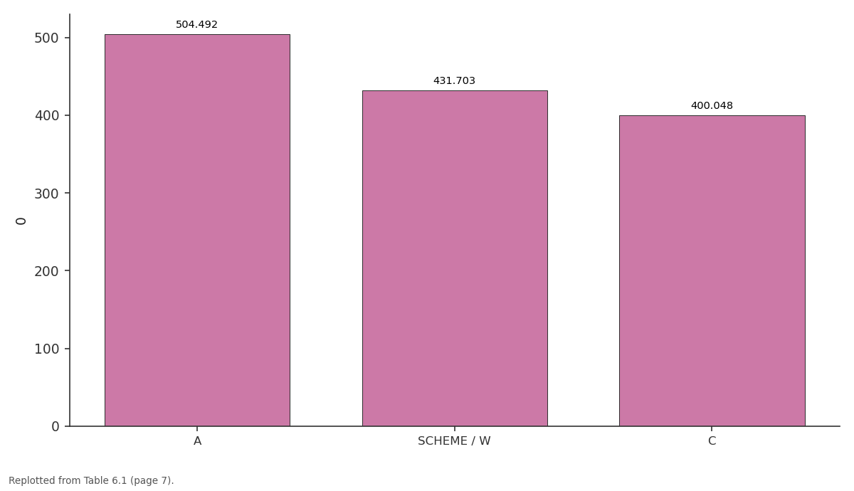
0: A vs SCHEME / W vs C
Replotted from Table 6 (page 7) of the original paper. Every bar is the paper's own table value.
View source evidence ↗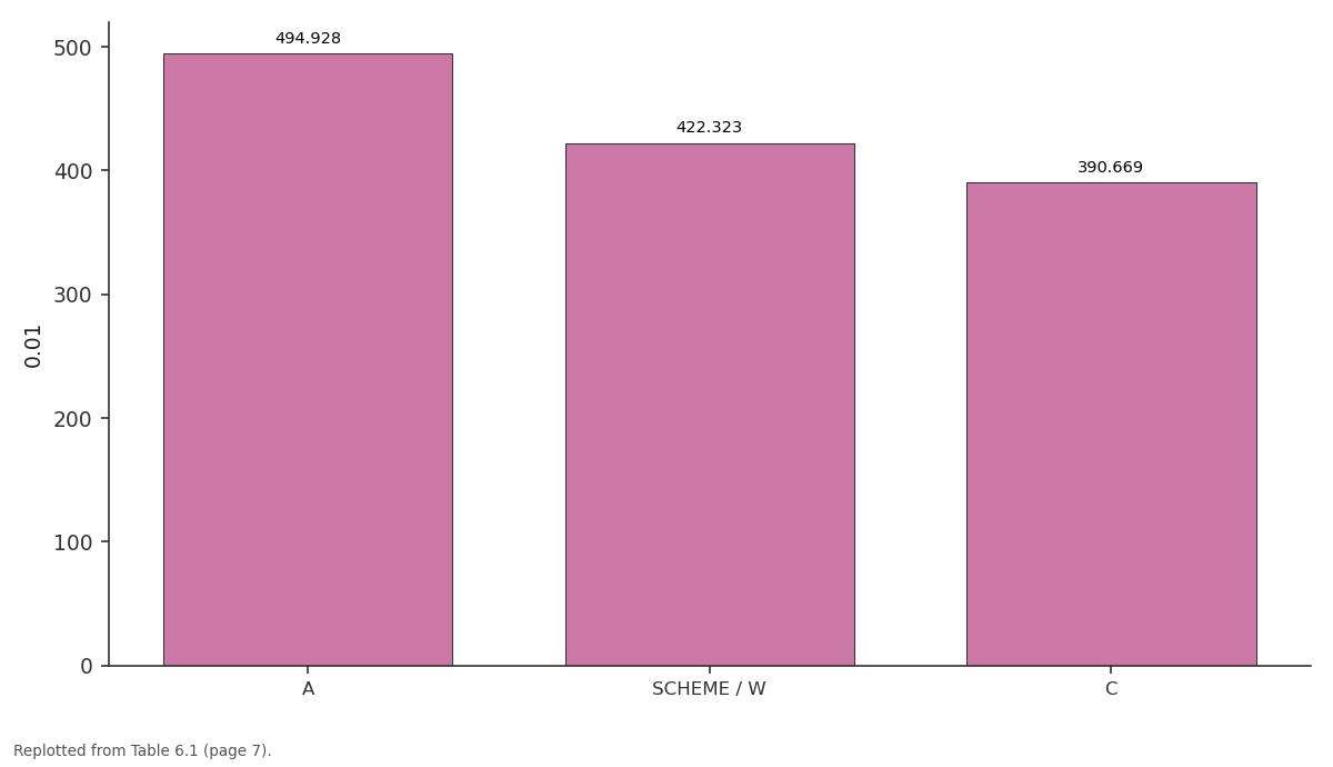
0.01: A vs SCHEME / W vs C
Replotted from Table 6 (page 7) of the original paper. Every bar is the paper's own table value.
View source evidence ↗Figures & tables
From the original paper Table 4
 Table 4
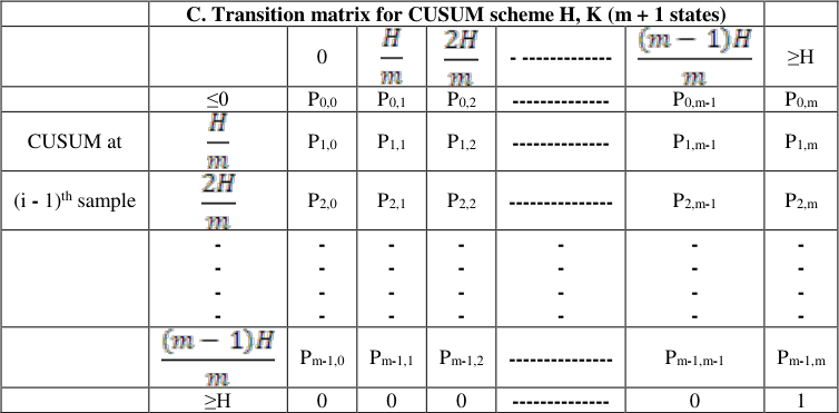 Table 4
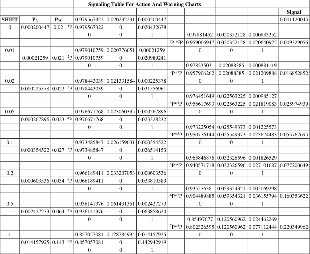 Table 5
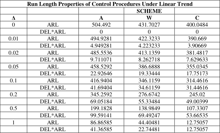 Table 6
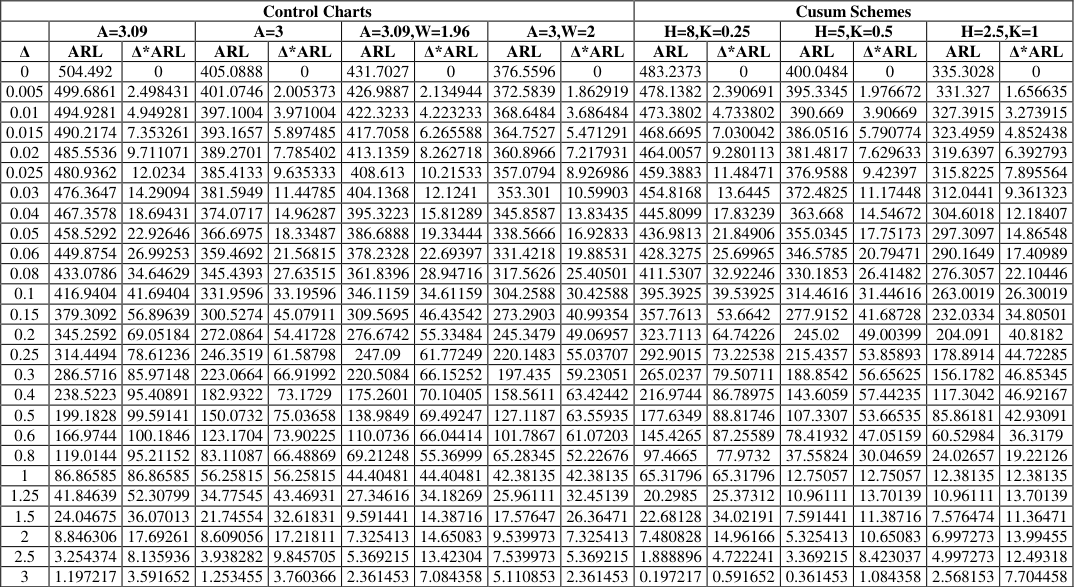 Table 6
Introduction
Cumulative Sum Schemes Control Charts were introduced in 1954 by Page (1954). These charts may be used in several situations where a production process is expected to change at an unknown time from an "in control state" to an "out of control state". As soon as one has evidence that the out of control state has observed one would wishes to stop the production process to take remedial measures. CUSUM schemes have proven to be optimal stopping rules in the sense that to minimize expected run length under the out of control state given that the stopping rules has a fixed expected run length under the in-control state Moustakides (1986) [10] . CUSUM control charts have found an interesting variety of applications since their introduction. Several researchers namely Johnson (1966) [7] , Hinkley (1970) [3] , Brook and Evans (1972) [1] , Ashish and Srivastava (1975) [14] , Hawkins (1977) [4] , Khan (1978) [8] , Koning and Does (1988) [9] , Rendtel (1990) [12] , Rogerson (2006) [13] , Cox (2009) [2] have attempted performance of CUSUM charts under various conditions. In most of the research problems the CUSUM chart performance is mainly assessed based on the Average Run Length or its distribution. In other words, the effectiveness of monitoring procedures like Shewart charts with Action limit only, control charts with Warning lines and CUSUM procedures can be demonstrated when there is a slippage in mean level from a target value. This can be done with the help of ARL or other features of run length distributions. The ARL is usually measured on the assumption of step change i.e. abrupt change from the process average. The main purpose of this paper is to assess the performance of control charts and CUSUM charts under linear trend with non-normal distribution namely, Rayleigh. This distribution and its importance is discussed as and when the CUSUM schemes and other control charts performance are assessed. In the subsequent sections we discuss Shewart chart with action line, control chart with warning line and CUSUM procedures.
Shewart Control Chart With Action Lines
In the construction of control charts we are using two sets of limits such as action limits or outer limits and warning limits or inner limits. When action lines point plots outside of this limit, a search for an assignable cause is made and corrective action is taken if necessary. Shewart control chart with only action lines, it is denoted by 'Scheme A' and specified distributional assumptions, the evaluation of run length properties follows Geometric distribution with parameter that is
Where is the Probability of action limit for a specified process mean.
Shewart Control Chart With Warning Lines
In a Shewart control chart with action and warning lines we take decisions with monitoring procedures depend on preceding observations as well as the most recent value. It is denoted by 'Scheme W'. If one or more points fall between the warning line and the central line or very close to the warning line, we should be suspicious that the process may not be operating properly. One possible action to take when this occurs is to increase the sampling frequency. The use of warning limit can increase the sensitivity of the control chart. The complete run length distribution is obtained by using successive powers of the transition matrix. In particular, the ARL is found to be
Where is the Probability of a violation of warning line which includes more extreme action line violation . The action line scheme is having only two states one Transient and another one is absorbing.
Properties
The raw moments are given by:
The mean and variance of a Rayleigh random variable may be expressed as:
The mode is σ and the maximum pdf is
If R is a Rayleigh then R 2 has a chi-square distribution with two degrees of freedom:
2 has a Gamma Distribution with Parameters N and 2σ 2 :
Parametric distributions are often used to model life time and time-to-failure responses. In statistical terminology, the Rayleigh distribution is a continuous distribution. For example, the Rayleigh distribution arises when the wind speed is studied with the acceleration of speed towards the orthogonal of two dimensional components. For all these cases we assume that each component is uncorrelated and normally distributed for equal variances. However, the entire phenomena i.e. speed is characterized by a Rayleigh distribution.
Transition Matrix for Control Chart
The Transition matrices representation for control charts are give below. In case of row labels refer to states at sample (i-1) and column heading to states at sample i. The upper left column partition is the reduced transition matrix after deleting row and column for the absorbing states.
Transition Matrix for Cusum Chart with Rayleigh Distribtuion
Brooks and Evans (1972) [1] show that CUSUM procedures may be viewed as Markov chains. However for, continuous distributions, it is necessary to consider the discretization for the markov chain representation and the various states then corresponds to values of the CUSUM at any step. For an instance consider a scheme with decision interval H and reference value K are designed to detect upward shift from a target value. A set of (m + 1) states can be interpreted as the CUSUM values of
The last of these states that is violation of the decision interval can be thought of as an absorbing barrier.
In the usual Markov chain notation with Transition matrix P and reduced matrix are one which is obtained from the deletion of the row and column representing the absorbing barrier. The well-known result for obtaining ARL from an initial zero CUSUM is the sum of the elements in the first row of . While considering the states the degree of discretization has some effect on the accuracy of ARL determination. In the present study 20 states transition matrices were used. Thus for H=5 and K=0.5 with μ at the target value. The transition matrix in general and for the particular study is shown in tables 4.3 and 5.1 respectively. -------------0 1
The entries in the above matrix need some explanation. In the first row, all entries corresponding moves from an initial zero CUSUM, and in the first entry, it indicates that a sample i, the CUSUM remains at or below zero. This means the sample value should not exceed the reference value k. Thus
For a move from state zero to H/m, the i th sample must have a value between K and (K +H/m). So that the subtraction of reference value gives a CUSUM contribution of H/m. After the discretization,
Run Length Calculation under Linear Trend with Rayleigh Distribution
The method explained for ARL calculations is applicable only under the assumption that the phenomenon or process average undergoes stable distribution. However, in case of liner trend both the distribution functions and transition matrix changes over the time. These changes can be quantifiable for any specific rate of slippage. Here we get a non-homogenous Markov chain and an alternative method of obtaining ARL is essential. This can be easily derived from the procedures for generalising run length distribution under stable conditions. The entry P0, m in the transition matrix stands for the probability of occurrence of a signal at the first sample instant. That means gives the probability of signal at the i th sample. For an increasing i, we get probability distribution of run length. For an illustration, consider W chart with action line at 3.09σe from a target value and warning limit at 1.96σe. Let the process changes to a value 1.00σe from the target value, then for Rayleigh variable
The transition matrix in this case is given by gives 0.0061690is the probability run length for three samples. In the case of non-homogenous transition matrix, it is necessary to multiply original P by new transition matrix obtained after allowing a step change in the mean level. We denote the rate of change by ∆ and we use 1 P, 2 P etc, for the first, second etc samples transition matrices are deduced. In general the Cumulative probability of signal at or before the i th sample is (0, m) th element of the product. i.e. 1 P 2 P 3 P-------i P Individual terms of the run length probability distribution are obtained by successive differences of cumulative probabilities. From the above calculations we get the cumulative probabilities of a signal at sample 2 is . Subtracting the (0, m) th element of 1 P gives 0.005475. The above computations are presented for the sake of illustration allowing slippages at different levels similar type of calculated and re-designated as 1 P 2 P 3 P -------For different slippages in mean level, say ∆ = 0.01, 0.02, 0.05, 0.1, 0.2 are computed and summarized below. In case of CUSUM scheme the transition matrix can be obtained by making use of the formulae given in section 4.3.3 these are summarised in the following matrix.
Run Length Properties of Standard Control Charts under Linear Trend with Rayleigh Distribution
The following table 6.1 gives the average run length and other properties of the run length distributions for three basic control charts namely A scheme, W scheme and CUSUM scheme. In these tables ∆ values ranges from 0 to 1. Here we note that the shift will be detected rapidly when the trend is greater than 1 standard error per sample in all chart methods. The entries in the third and fourth column are obtained by using equation ( 1) and ( 2) the first column ARL are obtained by using from initial zero CUSUM which is the sum of the elements in the first row of of respective slippage values. Here CUSUM scheme is operated with H = 5, K = 0.5 under Rayleigh distribution. The following table gives values of ARL and ∆*ARL (displacement ARL) for these basic control charts and the corresponding data for further two CUSUM scheme with H =8, K=0.25 and H=2.5, K=1
| Control Charts | — | — | — | — | — | — | — | — | Cusum Schemes | — | — | — | — | — |
|---|---|---|---|---|---|---|---|---|---|---|---|---|---|---|
| A=3.09 | A=3 | A=3.09,W=1.96 | A=3,W=2 | H=8,K=0.25 | H=5,K=0.5 | H=2.5,K=1 | ||||||||
| Δ | ARL | Δ*ARL | ARL | Δ*ARL | ARL | Δ*ARL | ARL | Δ*ARL | ARL | Δ*ARL | ARL | Δ*ARL | ARL | Δ*ARL |
| 0 | 504.492 | 0 | 405.0888 | 0 | 431.7027 | 0 | 376.5596 | 0 | 483.2373 | 0 | 400.0484 | 0 | 335.3028 | 0 |
| 0.005 | 499.6861 | 2.498431 | 401.0746 | 2.005373 | 426.9887 | 2.134944 | 372.5839 | 1.862919 | 478.1382 | 2.390691 | 395.3345 | 1.976672 | 331.327 | 1.656635 |
| 0.01 | 494.9281 | 4.949281 | 397.1004 | 3.971004 | 422.3233 | 4.223233 | 368.6484 | 3.686484 | 473.3802 | 4.733802 | 390.669 | 3.90669 | 327.3915 | 3.273915 |
| 0.015 | 490.2174 | 7.353261 | 393.1657 | 5.897485 | 417.7058 | 6.265588 | 364.7527 | 5.471291 | 468.6695 | 7.030042 | 386.0516 | 5.790774 | 323.4959 | 4.852438 |
| 0.02 | 485.5536 | 9.711071 | 389.2701 | 7.785402 | 413.1359 | 8.262718 | 360.8966 | 7.217931 | 464.0057 | 9.280113 | 381.4817 | 7.629633 | 319.6397 | 6.392793 |
| 0.025 | 480.9362 | 12.0234 | 385.4133 | 9.635333 | 408.613 | 10.21533 | 357.0794 | 8.926986 | 459.3883 | 11.48471 | 376.9588 | 9.42397 | 315.8225 | 7.895564 |
| 0.03 | 476.3647 | 14.29094 | 381.5949 | 11.44785 | 404.1368 | 12.1241 | 353.301 | 10.59903 | 454.8168 | 13.6445 | 372.4825 | 11.17448 | 312.0441 | 9.361323 |
| 0.04 | 467.3578 | 18.69431 | 374.0717 | 14.96287 | 395.3223 | 15.81289 | 345.8587 | 13.83435 | 445.8099 | 17.83239 | 363.668 | 14.54672 | 304.6018 | 12.18407 |
| 0.05 | 458.5292 | 22.92646 | 366.6975 | 18.33487 | 386.6888 | 19.33444 | 338.5666 | 16.92833 | 436.9813 | 21.84906 | 355.0345 | 17.75173 | 297.3097 | 14.86548 |
| 0.06 | 449.8754 | 26.99253 | 359.4692 | 21.56815 | 378.2328 | 22.69397 | 331.4218 | 19.88531 | 428.3275 | 25.69965 | 346.5785 | 20.79471 | 290.1649 | 17.40989 |
| 0.08 | 433.0786 | 34.64629 | 345.4393 | 27.63515 | 361.8396 | 28.94716 | 317.5626 | 25.40501 | 411.5307 | 32.92246 | 330.1853 | 26.41482 | 276.3057 | 22.10446 |
| 0.1 | 416.9404 | 41.69404 | 331.9596 | 33.19596 | 346.1159 | 34.61159 | 304.2588 | 30.42588 | 395.3925 | 39.53925 | 314.4616 | 31.44616 | 263.0019 | 26.30019 |
| 0.15 | 379.3092 | 56.89639 | 300.5274 | 45.07911 | 309.5695 | 46.43542 | 273.2903 | 40.99354 | 357.7613 | 53.6642 | 277.9152 | 41.68728 | 232.0334 | 34.80501 |
| 0.2 | 345.2592 | 69.05184 | 272.0864 | 54.41728 | 276.6742 | 55.33484 | 245.3479 | 49.06957 | 323.7113 | 64.74226 | 245.02 | 49.00399 | 204.091 | 40.8182 |
| 0.25 | 314.4494 | 78.61236 | 246.3519 | 61.58798 | 247.09 | 61.77249 | 220.1483 | 55.03707 | 292.9015 | 73.22538 | 215.4357 | 53.85893 | 178.8914 | 44.72285 |
| 0.3 | 286.5716 | 85.97148 | 223.0664 | 66.91992 | 220.5084 | 66.15252 | 197.435 | 59.23051 | 265.0237 | 79.50711 | 188.8542 | 56.65625 | 156.1782 | 46.85345 |
| 0.4 | 238.5223 | 95.40891 | 182.9322 | 73.1729 | 175.2601 | 70.10405 | 158.5611 | 63.42442 | 216.9744 | 86.78975 | 143.6059 | 57.44235 | 117.3042 | 46.92167 |
| 0.5 | 199.1828 | 99.59141 | 150.0732 | 75.03658 | 138.9849 | 69.49247 | 127.1187 | 63.55935 | 177.6349 | 88.81746 | 107.3307 | 53.66535 | 85.86181 | 42.93091 |
| 0.6 | 166.9744 | 100.1846 | 123.1704 | 73.90225 | 110.0736 | 66.04414 | 101.7867 | 61.07203 | 145.4265 | 87.25589 | 78.41932 | 47.05159 | 60.52984 | 36.3179 |
| 0.8 | 119.0144 | 95.21152 | 83.11087 | 66.48869 | 69.21248 | 55.36999 | 65.28345 | 52.22676 | 97.4665 | 77.9732 | 37.55824 | 30.04659 | 24.02657 | 19.22126 |
| 1 | 86.86585 | 86.86585 | 56.25815 | 56.25815 | 44.40481 | 44.40481 | 42.38135 | 42.38135 | 65.31796 | 65.31796 | 12.75057 | 12.75057 | 12.38135 | 12.38135 |
| 1.25 | 41.84639 | 52.30799 | 34.77545 | 43.46931 | 27.34616 | 34.18269 | 25.96111 | 32.45139 | 20.2985 | 25.37312 | 10.96111 | 13.70139 | 10.96111 | 13.70139 |
| 1.5 | 24.04675 | 36.07013 | 21.74554 | 32.61831 | 9.591441 | 14.38716 | 17.57647 | 26.36471 | 22.68128 | 34.02191 | 7.591441 | 11.38716 | 7.576474 | 11.36471 |
| 2 | 8.846306 | 17.69261 | 8.609056 | 17.21811 | 7.325413 | 14.65083 | 9.539973 | 7.325413 | 7.480828 | 14.96166 | 5.325413 | 10.65083 | 6.997273 | 13.99455 |
| 2.5 | 3.254374 | 8.135936 | 3.938282 | 9.845705 | 5.369215 | 13.42304 | 7.539973 | 5.369215 | 1.888896 | 4.722241 | 3.369215 | 8.423037 | 4.997273 | 12.49318 |
| 3 | 1.197217 | 3.591652 | 1.253455 | 3.760366 | 2.361453 | 7.084358 | 5.110853 | 2.361453 | 0.197217 | 0.591652 | 0.361453 | 1.084358 | 2.568153 | 7.704458 |
Table text extracted from the original PDF; superscript letters are shown inline. The original table image is below.
View original table image
| Run Length Properties of Control Procedures Under Linear Trend | — | — | — | — |
|---|---|---|---|---|
| SCHEME | ||||
| Δ | A | W | C | |
| 0 | ARL | 504.492 | 431.7027 | 400.0484 |
| DEL*ARL | 0 | 0 | 0 | |
| 0.01 | ARL | 494.9281 | 422.3233 | 390.669 |
| DEL*ARL | 4.949281 | 4.223233 | 3.90669 | |
| 0.02 | ARL | 485.5536 | 413.1359 | 381.4817 |
| DEL*ARL | 9.711071 | 8.262718 | 7.629633 | |
| 0.05 | ARL | 458.5292 | 386.6888 | 355.0345 |
| DEL*ARL | 22.92646 | 19.33444 | 17.75173 | |
| 0.1 | ARL | 416.9404 | 346.1159 | 314.4616 |
| DEL*ARL | 41.69404 | 34.61159 | 31.44616 | |
| 0.2 | ARL | 345.2592 | 276.6742 | 245.02 |
| DEL*ARL | 69.05184 | 55.33484 | 49.00399 | |
| 0.5 | ARL | 199.1828 | 138.9849 | 107.3307 |
| DEL*ARL | 99.59141 | 69.49247 | 53.66535 | |
| 1 | ARL | 86.86585 | 44.40481 | 12.75057 |
| DEL*ARL | 41.36585 | 22.74481 | 12.75057 |
Table text extracted from the original PDF; superscript letters are shown inline. The original table image is below.
View original table image
Conclusions
The various control schemes considered here are, in effect, continuous hypothesis tests. These hypotheses can be stated as In real world, it is frequently unknown whether the process averages μ will change suddenly or gradually. Most of the ARL calculations are based on the one standard deviation schemes under a trend alternative.
If trend is expected in the process average, this prior knowledge will be incorporated in to the design of control procedures while considering sampling intervals.
In the case of Rayleigh distribution suggest that there exists less difference in performance among schemes A, W and C under the linear trend than under step change conditions. Where as in scheme C with Rayleigh distribution the lower ARL for slippage of 0.2 to 0.1 standard errors is noted. It can be observed that the standard C scheme with Rayleigh distribution gives somewhat quicker response over the range 0.015 ≤ ∆ ≤ 0.6 as compared with schemes of A and W schemes over the range 0.03 ≤ ∆ ≤ 0.3. These results are broadly compatible for those relating to step changes, in that, for example with ARL ≅ 6, at ∆ = 0.3 for W and C schemes, the process mean must have shifted above two standard errors by the time the trend is detected. Similarly, for A and C shift is about 3 standard error with ARL ≅ 4.9 at ∆= 0.6. For step changes greater than 2.5 , it is observed that lower ARL for W when compared with C scheme. The same situation is prevailed in the case of slippage greater than 2.5 . In table 6.2, the values of ∆ ARL gives for further clarification on the point of selection A, W and C alternatives.
Figures and tables from the paper
| A. Transition matrix for "Action only" (Shewart) chart | — | — |
|---|---|---|
| clear | signal | |
| clear | 1-PA | PA |
| signal | 0 | 1 |
Table text extracted from the original PDF; superscript letters are shown inline. The original table image is below.
View original table image
| W. Transition matrix for "Action and Warning" control chart | — | — | — |
|---|---|---|---|
| clear | Warning | signal | |
| clear | 1-PA | PW-PA | PA |
| Warning | 1-PW | 0 | PW |
| Signal | 0 | 0 | 1 |
Table text extracted from the original PDF; superscript letters are shown inline. The original table image is below.
View original table image
| — | C. Transition matrix for CUSUM scheme H, K (m + 1 states) | — | — | — | — | — | — |
|---|---|---|---|---|---|---|---|
| 0 | - ------------- | ≥H | |||||
| ≤0 | P0,0 | P0,1 | P0,2 | -------------- | P0,m-1 | P0,m | |
| CUSUM at | P1,0 | P1,1 | P1,2 | -------------- | P1,m-1 | P1,m | |
| (i - 1)th sample | P2,0 | P2,1 | P2,2 | --------------- | P2,m-1 | P2,m | |
| - - - - | - - - - | - - - - | - - - - | - - - - | - - - - | - - - - | |
| Pm-1,0 | Pm-1,1 | Pm-1,2 | --------------- | Pm-1,m-1 | Pm-1,m | ||
| ≥H | 0 | 0 | 0 | -------------- | 0 | 1 |
Table text extracted from the original PDF; superscript letters are shown inline. The original table image is below.
View original table image
| — | — | — | — | Signaling Table For Action And Warning Charts | — | — | — | — | — | — | — |
|---|---|---|---|---|---|---|---|---|---|---|---|
| Signal | |||||||||||
| SHIFT | PA | PW | 0.979567322 | 0.020232231 | 0.000200447 | 0.001120045 | |||||
| 0 | 0.000200447 | 0.02 | 1P | 0.979567322 | 0 | 0.020432678 | |||||
| 0 | 0 | 1 | 0.97881452 | 0.020352128 | 0.000833352 | ||||||
| 1P *2P | 0.959006947 | 0.020352128 | 0.020640925 | 0.009329056 | |||||||
| 0.01 | 0.979010759 | 0.020776651 | 0.00021259 | 0 | 0 | 1 | |||||
| 0.00021259 | 0.021 | 2P | 0.979010759 | 0 | 0.020989241 | ||||||
| 0 | 0 | 1 | 0.978235031 | 0.02088385 | 0.000881119 | ||||||
| 2P*3P | 0.957906262 | 0.02088385 | 0.021209888 | 0.016852852 | |||||||
| 0.02 | 0.978443039 | 0.021331584 | 0.000225378 | 0 | 0 | 1 | |||||
| 0.000225378 | 0.022 | 3P | 0.978443039 | 0 | 0.021556961 | ||||||
| 0 | 0 | 1 | 0.976451649 | 0.022563225 | 0.000985127 | ||||||
| 3P*4P | 0.955617693 | 0.022563225 | 0.021819083 | 0.025974939 | |||||||
| 0.05 | 0.976671768 | 0.023060335 | 0.000267896 | 0 | 0 | 1 | |||||
| 0.000267896 | 0.023 | 4P | 0.976671768 | 0 | 0.023328232 | ||||||
| 0 | 0 | 1 | 0.973225054 | 0.025549373 | 0.001225573 | ||||||
| 4P*5P | 0.950776144 | 0.025549373 | 0.023674483 | 0.055767695 | |||||||
| 0.1 | 0.973485847 | 0.026159631 | 0.000354522 | 0 | 0 | 1 | |||||
| 0.000354522 | 0.027 | 5P | 0.973485847 | 0 | 0.026514153 | ||||||
| 0 | 0 | 1 | 0.965846876 | 0.032326596 | 0.001826529 | ||||||
| 5P*6P | 0.940571718 | 0.032326596 | 0.027101687 | 0.077200649 | |||||||
| 0.2 | 0.966189411 | 0.033207053 | 0.000603536 | 0 | 0 | 1 | |||||
| 0.000603536 | 0.034 | 6P | 0.966189411 | 0 | 0.033810589 | ||||||
| 0 | 0 | 1 | 0.935576381 | 0.059354321 | 0.005069298 | ||||||
| 6P*7P | 0.904489885 | 0.059354321 | 0.036155794 | 0.160353622 | |||||||
| 0.5 | 0.936141376 | 0.061431351 | 0.002427273 | 0 | 0 | 1 | |||||
| 0.002427273 | 0.064 | 7P | 0.936141376 | 0 | 0.063858624 | ||||||
| 0 | 0 | 1 | 0.85497677 | 0.120560962 | 0.024462269 | ||||||
| 7P*8P | 0.802326595 | 0.120560962 | 0.077112444 | 0.220349962 | |||||||
| 1 | 0.857057081 | 0.128784994 | 0.014157925 | 0 | 0 | 1 | |||||
| 0.014157925 | 0.143 | 8P | 0.857057081 | 0 | 0.142942919 | ||||||
| 0 | 0 | 1 |
Table text extracted from the original PDF; superscript letters are shown inline. The original table image is below.
View original table image
References
14 in the original paper- Brook D, Evans DA. An approach to the probability distribution of Cusum run length, Biomertika, 1972, 59.
- Cox MAA. A comparison of Formulas for the design of cumulative sum control charts. Quality Reliability Engineering. 2009; 25:731-737.
- Hinkley DV. Inference about the change point in a sequence of random variables. Biomertika. 1970; 57:1-17.
- Hawkins DM. Testing a sequence of observations for a shift in location. Journal of the American Statistical Association. 1977; 72:180-186.
- Johnson NL. Cumulative sum control charts and the Weibull Distribution. Technometrics. 1966; 8:481-491.
- James Benneyan C. Performance of Number-Between g-Type Statistical Control Charts for Monitoring Adverse Events. Health Care Managemen Science. 2001; 4:319-336.
- Johnson NL. Cumulative sum control charts and the Weibull Distribution. Technometrics. 1966; 8:481-491.
- Khan RA. Wald's approximations to the average run length in CUSUM procedures. Statist. Plan. And Inf. 1978; 2:63-77.
- Koning AJ, Does RJMM. Cusum charts for preliminary analysis of individual observations. Manuscript, submitted for publication. 1988; 3:133-137.
- Moustakides GV. Optimal Stopping Times for detecting changes in distributions. Ann. Statist. 1986; 14:1379-1387.
- Page ES. Continuous inspection schemes. Biometrika. 1954; 41:100-114.
- Rendtel U. Cusum schemes with variable sampling intervals and sample sizes. Statistical papers, Springer Verlag. 1990; 31:103-118.
- Rogerson PA. Formulas for the design of CUSUM quality control charts. Communications in Statistics-Theory and Methods. 2006; 35:373-383.
- Sen A, Srivastava MS. On tests for detecting change in mean when variance is unknown. Annuals of the Institute of Statistical Mathematics. 1975; 27:479-486.