Choice of optimum design and procedures ensuring in reliability analysis

The concept of reliability has been interpreted in many different ways in numerous works. In different fields of application the concept of reliability is interpreted in many different ways. One of the definitions which has been accepted by most contemporary reliability authorities is given by the Electronic Industries Association (EIA) of USA which states as “Reliability is the probability of an item performing its intended function or a given period of time under the operation conditions encountered”.

Illustrations explain the paper; charts are replotted from the paper's own table values.

AI-generated illustration

↗ Enlarge

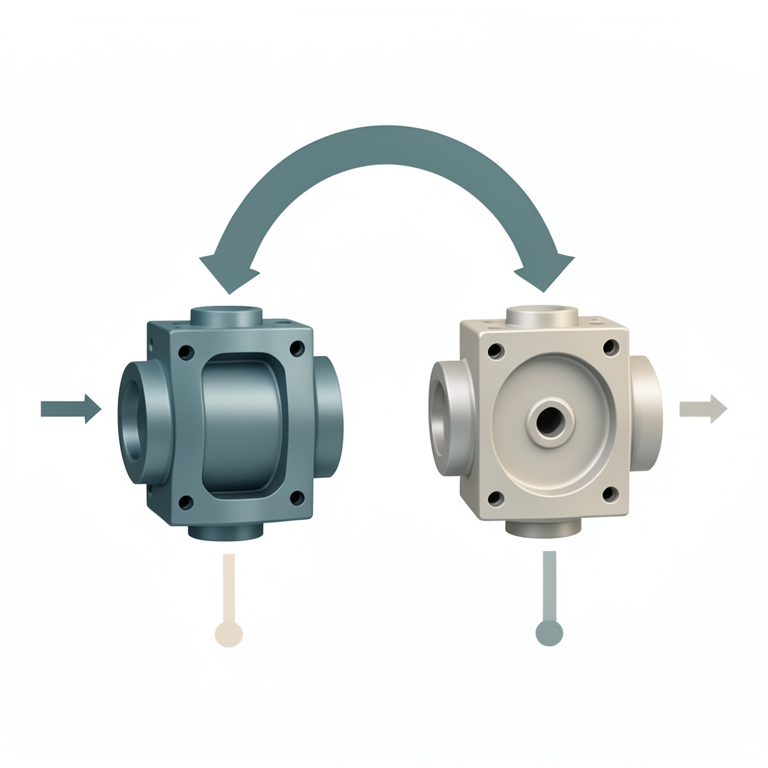
LCCS Series System ConceptClose ×

AI-generated conceptual illustration (two distinct industrial mechanical components in a series configuration). It explains the idea and does not show study data.

Open full-size image ↗

Replotted from source data

↗ Enlarge

0: β = 0.0 / W= 0.0 vs β = 0.1 / W= 0.1 vs β = 0.2 / W= 0.2 vs β = 0.3 / W= 0.3Close ×

Replotted from a table (page 6) of the original paper. Every bar is the paper's own table value.

Open full-size image ↗

Replotted from source data

↗ Enlarge

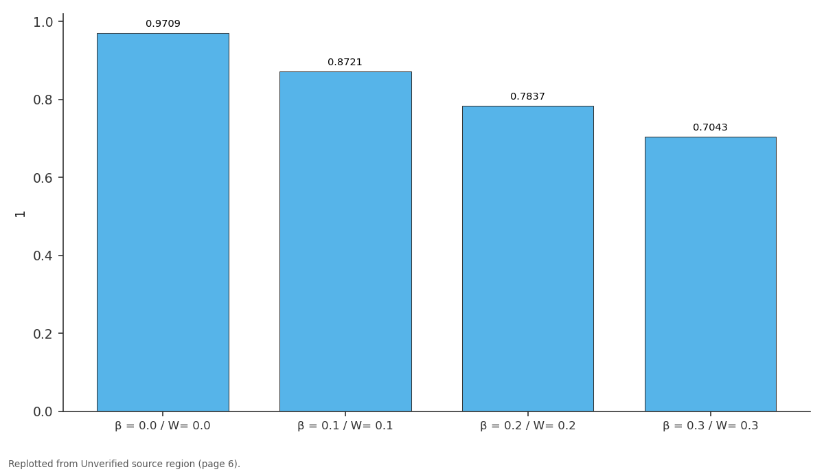
1: β = 0.0 / W= 0.0 vs β = 0.1 / W= 0.1 vs β = 0.2 / W= 0.2 vs β = 0.3 / W= 0.3Close ×

Replotted from a table (page 6) of the original paper. Every bar is the paper's own table value.

Open full-size image ↗

Introduction

Reliability is a new branch of activity, which figured during world war II and deals with integral features of the planning, design, testing, manufacture, acceptance and use of products to obtain the 'effectiveness' of the products. The theory of reliability had been developed during the last five decades. Available contribution was made to the development of the theory of reliability by the mathematicians of the like Gnedenkov, Belyayev, Solovyev, plovoko, Barlow and proschan. The development of present day technology created special attention toward numerous problems concerning the improvement of the 'effectiveness' of the products. The 'effectiveness' or 'efficiency' of a system is understood to mean the combination of properties that determine the degree of suitability of the system for the fulfillment of the task. Sometimes this is also referred to 'qulity'in the literature. The efficiency of the system which is performing a specific task, is described by the terms such as reliability, survivability. Reliability means the ability of the system to perform its intended function satisfactorily. The term reliability as defined by AGREE [1] (Advisory group on Reliability of Electronic Equipment) is the probability that device/system will perform its intended function adequately over a period of time Unser the specified operating conditions. In otherwords, it is the probability of the system's or device's 'uninterrupted working' or 'trouble-free' working in a specified period of time. The concept of 'survivability' is understood as the ability of the system to preserve the properties to serve its purpose under adverse conditions (viz. explosions, fire, inundation etc…). The reliability of a system is in turn determined by more concrete properties of the system, namely 'trouble-proofness' is the property of a system to preserve its capability in the duration of a definite time under the normal conditions of function. Reparability (restorability) means the suitability of a system for a the prevention, detection and elimination of failures. 'Longevity' id the ability for a prolonged operation with the necessary technical maintenance including various kinds of repairs. 'Maintainability' is define as the probability that failed equipment is restored to operable condition in a specified time (know as down time). How often an equipment fails and how long it is down' are the vital consideration in determining of repairable equipment's. It is the combination of 'reliability' and 'maintainability'. 'Failure' plays an important role in the context of reliability assessment. 'Failure' is an event after which a system is incapacitated. In the reliability theory 'failure' is define as the termination of ability of satisfactory performed of a system. The notion of failure is a useful characteristic of reliability analysis because it is mainly responsible for various numerical criteria of reliability analysis.

The objective of reliability theory is to establish and study the characteristics of reliability and to investigate the connection between the indices of efficiency, reliability and economy of the systems. In reliability theory one is interested with the following. 1) Development of methods for evaluation of reliability characteristics. 2) Development of methods for establishing rules and choices of characteristics ensuring optimum reliability.

3) Development of methods of choice of optimum design and procedures ensuring a given reliability methods.

The requirement that devices or systems of various types function without failure is required for all technological devices. For instance, one is interested always with the questions like: i. What is the use of an aircraft that cannot complete a flight without failure? ii. What is the use of a tractor that cannot perform the work for which it is meant for or an automobile that cannot transport goods or passengers One is interested in the problem of unreliability of the products he is using. The important of unreliability and problems he is using regarding it is very much concerned in the theory of reliability.

In this chapter we will be concerned with the determination of the reliability characteristic i.e. Reliability (RHI) and mean time between failures (MTBF) which reveals the important measures of the effectiveness of the system in the reliability analysis. In the present chapter, the emphasis is on the Markovian Approach for lethal common cause Shock (LCCS) failures in order to derive the important reliability characteristics which are mentioned already in our previous chapter. We consider when the system is influenced by lethal shocks in addition to individual failures along with non-lethal common cause shock failures. We referred this type of model is as lethal common cause shock failures model (LCCS model) in this research work.

The expressions for Reliability function and mean time between failures of the system under the influence of lethal common cause shock failures for mathematical models were developed. Also we compare the reliability and MTBF of the system in the presence of Lethal common. Cause shock failures that of the situation when only individual failures are effecting the system.

For the present study, two s-independent and non-identical components were considered and the results of the Reliability and MTBF of the system for series configuration are discussed and presented in this chapter. a) Reliability is the integral of the distribution of probabilities of failure-free operation from the instant of switch-on to the first failure. b) The reliability of a component (or a system) is the probability that the component (or the system) will not fail for a time 't' c) The reliability is the mean operating time of a given specimen between two failures. d) The reliability of a system is called its capacity for failure-free operation for a definite period of time under the given operating conditions and for minimum time lost for repair and preventive maintenance. e) The reliability of equipment is arbitrarily assumed to be the equipment capacity to maintain given properties under specified operating conditions and for a given period time.

The failure is defined as the inability of equipment not to breakdown in operation.

Measures of Raliability

The prediction of system reliability is based on number of factors, such as life characteristics, operating conditions and the failure distribution. Thus, the initial step in reliability predictions the determination of life characteristics. If a random sample of items are taken from a population and are put to test (or use) under a set of fixed (or given) environmental or operating conditions the members of the sample will fail successively in time. The data so obtain will represent the life length of each item. The life length can be measured depending on whether the item is repairable or non-repairable. For repairable items, the life can be measured by failure rate or mean time between failures; where as for non-repairable items, the life can be measured y mean time to failure.

Failure Rate

The failure rate is denoted by r, and it is expressed in terms of failures per 100 or 1000 hours. It is computed as a simple ratio of number of failures, N, during a specified test interval, to the total test time o the items under going test. Thus,

Where, r = failure rate N = number of failures fueing the test interval T = Total test time.

When the design in mature, the failure rate is fairly constant during the operating or useful life of the system. The smaller the value of the failure rate, the higher is the reliability of the system.

Mean Time between Failures (MTBF)

During the operating period, when failure rate is fairly constant, the mean time between failures (MTBF) is the reciprocal of the constant failure rate or the ratio of the test time to the number of failures

Mean time between failures is also referred as the average time os satisfactory operation of the system. In this case, larger the MTBF, higher is the system. Generally, the failure rate and mean time to failure are used where the item is repairable.

Mean Time to Failure (MTTF)

The mean time to failure is applicable to non-repairable items. The mean time to failure is expressed as the average time an item may be expected to function before failure. If we have a life test information on 'n' items with failure items t 1 , t 2 , t n then (MTTF) is defined as

Probability of Survival

The probability of survival is expressed as a decimal fraction or percentage which indicates the probable or expected number of items that will operate for a required period of time.

Derivation of Reliability Function

If an event can occur in N mutually exclusive and equally likely ways, n of which possesses the characteristics A, and m of which do not have the characteristic A, then the probability of a occurring is n/N. Symbolically,

We will now translate this concept for the reliability of a component. Let a fixed number N, of components be repeatedly tested. There will be, after a time t, n components which survive the test and m components which will fail. Therefore, N = (n + m) is test because as the test proceeds, the number of failed components 'm' increases exactly as the number of surviving components 'n' decreases. The reliability (or probability of survival) expresses as a fraction of what (by the probability definition), at any time't', during the test is

Where n or m are counted at a specific time, t. The probability of failure or UN reliability at any time, t can be expressed as

Because R (t) and F (t) are mutually exclusive events. The equation ( 5) can also be written as

Differentiating the equation ( 8) with respect to t, we have

Which is the rate at whci components fail? Since, m = (Nm), we get an differentiation

The equation (11) indicates the negative rate at which the components scurvies. The term dt dm can be interpreted as the number of components failing in the time interval dt between the times t and t + dt. which is equivalent to the rate at which the component population still in test at time t, is failing. Dividing equation (10) by n both sides, we have

The left hand side of the equation ( 12) is the failure rate, r (t) and

By rearranging equation ( 13) and integrating with proper limits, we have

Initially, at t = 0, we have R (t) = 1 Therefore, (16) This gives a general formula for computing reliability. In equation ( 16), r (t) is a constant over time, and let r (t) = r say, then the reliability formula (16) becomes

Failure and Its Causes

For each item, the properties that it must posses in the course of its use are listed. A deviation in the properties of the item from the prescribed conditions is considered as a fault. A state of fault is denoted by the term "failure". An item is considered to have failed under one of the three conditions: (i) When it becomes completely inoperable.

(ii) When it is still operable but is no longer able to perform its intended function satisfactorily. Or (iii) When serious deterioration has made it unable or unsafe for continued use, and thus necessitating its immediate removal from service for repair or replacement.

The fundamental sources of failure include many aspects of design, material selection, material imperfections, fabrication and processing, reworking, assembly, inspection, testing, quality control, storage and shipment, service conditions, maintenance and un anticipated exposure to over load or mechanical or chemical change in service, often, more than one source contributes to the occurrence of a given failure. The measure of a system's reliability is the frequency at each failures occurs. If there no failure, the system is considered reliable.

If the failure frequency is very low, the system reliability is usually still acceptable, where as if the failure frequency is high the system is considered to be unreliable.

For the enhancement of system reliability, it is necessary that the design engineer understands the causes of failures, so as to the deficiency and discrepancy, if any, in the system. The primary concern is to recognize the causes of failures and to take corrective action so as to achiever higher system reliability. A few of the major causes which give rise to failure are (I) Deficiencies in design, (II) Deficiencies in material, (III) Deficiencies in processing, (IV) Errors in Assembly, (V) Improper service conditions and (IV) Inadequate maintenance.

Modes of Failures

In this section, we will discuss very briefly the manner in which system failures occur, so that appropriate corrective measures can be taken.

Catastrophic Failures

A catastrophic failure causes a normally operating system to suddenly become in operative. For example, a blow fuse or a random 'operation' occurring in a wire resister after several hundred hours of operation. This type of failure occurs at random and we can statistically predict the probability of occurrences of one or more catastrophic failures for any time period, if we know the failure rate,

Degradation (Creedpin) Failures

These are the type of failures which occur gradually because of the chance of some parameter with time. For example, a decrease in the value of a Tran's conductance in a radio tube will cause a drop in power output. A chance in the value of the resistance of a resistor might cause excessive frequency shift in the receiver. These failures can be detected and weeded out by proper inspection and maintenance.

Independent Failures

An independent failure may be of the catastrophic degradation or wear-out type. It is called independent as it does not occur as a result of the effects generated by other failures. For example, the failure of the fan-belt of an automobile is not related in any manner to the puncturing of the type of the wheel.

Secondary Failures

A secondary failure occurs as a result of some primary failure. For example, the spokes in the motor cycle traveling at high speed are broken as a result of a type burst. The braking of spokes would be considered as a secondary failure. On the other hand, if a resister in an electronic circuit is shorted thereby causing an excessive drain on the tube. The tube failure would then the secondary failure.

Lccs Model Reliability of Series Configuration

If the two component no-identical system under consideration is a series one, then the states one, two and three are considered to be dead states and hence transition from states on, two and three to zero state do not exist. (i.e. μ 0 = μ 1 = 0) Therefore the Reliability of the series system for the LCCS model is

 1 ,  2 ,  3 in the above expression, the quantities that appear in the expressions ( 19) & (20) are to be seen as A = 2{λ 1 + β P The formula for reliability or the series system in the cause of LCCS failures agree with the result of CHARI [10] for identical two compound system by letting λ 1 = λ 2 = λ and P 1 = P 2 = P in expression Also The expression après with the individuals failures (?) in the case of identical components, if we assume that the LCSS as well as NCCS failures do not occur (i.e  =w=o)

LCCS model -MTBF of the Series System

For two components non-identical series system, the expected life (or) the average time during which an item performs its function successfully In the case of LCCS failures model is derived as

[l 1 exp (  1 t) -l 2 exp (  2 t) + l 3 exp (  3 t)]dt.

= (l 2 /  2 ) -(l 1 /  1 ) + (l 3 /  3 )

Numerical Results

The Values of reliability in the series configuration is obtained as a function of time 't' taking the failure rates as λ 1 = 0.01 failure/ hr., λ 2 = 0.02 failures/hr., with P 1 = 0.03 and P 2 = 0.04 for various values of lethal and non-lethal common cause shock failure, and are shown in table 3

1. Barlow RE, Proschan F. Mathematical Theory of Reliability, John wiley, Now York, 1965.
2. Berg M. A proof of optimality for Age Replacement Policies, J Appl. Prob. 1976; 13(3):751-759.
3. Billinton R, Maccormack TKP. HAMS Spare component Management Evaluation in Reliability and Availability Studies. Proc. Engineering Conf. Reliability for the Electroni Power System Industry, 1982.
4. Billinton R, Medicheral TK. Application of Common Cause outage models in composite system And Sachdev, MS. Reliability evaluation, IEEE Trans. On Power Apparatus and System. 1981; 100:3648-3659.
5. Brown. Decision Rules for ventory Management, Englewood Cliff, NJ, 1967.
6. Campbell NR. The Replacement of Perishable Numbers of a continually operating System, J Roy, Stat. Soc. 1941; 7:110-130.
7. Chung WK. An Availability Calculation for K-Our-Of-N Redundant System with Common-Cause Failures and Replacement, Microelectron, Re; oab. 1980; 20:517-519.
8. Chae KC. System Reliability in the Presence of Common-Cause Failures, IEEE Trans. On Reliability. 1986; 35:32-35.
9. Cohen A. Morris Joint Pricing and ordering policy for exponentially decaying Inventory with known demand, Nov. Res. Log. Q. 1977; 24(2):257-268.
10. Dhillon BS. A 4-Unit Redundant System with Common-Cause Failures, IEEE Transactions on Reliability. 1977; 26(5):373374.
11. Drink water RW, hasting NAJ. An Economic Replacement Model, Opl. Res. Quar. 1967; 18:121-138.
12. Edward Silver A. A single method of determining order Quantities in joint replenishments under deterministic demand, Mgt. Sci. 1976; 22:12.
13. Elton EJ, Gruber NJ. On the optimality of an equalize policy for equipment subject to technological improvement, Op. Res. Quar. 1979; 27:93-98.
14. Ghare PM, Schrader GF. A model for exponential decaying Inventory, Jou. Ind. Engg. 1963; 14(5):238-243.
15. Hadley G, whitin JM. Analysis of Inventory Systems, Prentice-Hall, Englewood Cliffs, NJ, 1963.
16. Lotka AJ. A contribution to the theory of self-Renewing aggregated with special Reference to Industrial replacement, Am. Math. Slat. 1939; 10:1-25.