
Research article · 2018 · Full text
International Journal of Statistics and Applied MathematicsSARIMA models forecasting of weather parameters for Thrissur district
Volume 3(1) · Pages 360–367
Research areasAgricultural Economics and PracticesForecasting Techniques and ApplicationsHydrological Forecasting Using AI
Abstract
Author-writtenA novel attempt has been made to construct prediction models for weather parameters of Thrissur District in Kerala using SARIMA (Seasonal Auto Regressive Integrated Moving Average) models. Assessment of trend and identification of the best SARIMA model for forecasting weather in Thrissur District were the major objectives of the study. Excellent parsimonious forecasting equations could be generated using the SARIMA technique for the parameters studied. Validity of the models was tested using standard statistical techniques. The forecasting power of SARIMA model was used to forecast six leading years and the forecasted values are recorded. The results showed good agreement between actual and predicted values.
Summary
Source-checkedPlain-language reading of the full paper, prepared with AI and checked against the text. Each point links to the authors' own words.
Why it matters
- Global climate change and variability have led to an increase in weather-related disasters such as floods, droughts, and heat waves worldwide. View evidence ↗
- In Kerala, India, the India Meteorological Department reported increases in mean maximum (0.8 °C), mean minimum (0.2 °C), and average temperatures (0.5 °C) from 1961 to 2003. View evidence ↗
- Kerala has experienced a declining trend in annual rainfall over the last six decades, particularly during the southwest monsoon. View evidence ↗
The question
- The study aimed to assess weather trends and identify the most effective SARIMA models for forecasting weather parameters in the Thrissur District. View evidence ↗
What they did
- Daily weather data for the Thrissur District were collected from the Principal Agro-meteorological Observatory at Kerala Agricultural University for the period 1983 to 2015. View evidence ↗
- The analyzed parameters included maximum and minimum temperature, humidity and cloud hours (at 7 am and 2 pm), total rainfall, number of rainy days, and wind speed. View evidence ↗
- The researchers calculated monthly means from the daily weather observations to use in their models. View evidence ↗
- Model selection was based on diagnostics including R², AIC/BIC, RMSE, MAE, and MAPE. View evidence ↗
What they found
- For maximum temperature, the SARIMA (0, 0, 2) (0, 1, 1)12 model was best, explaining 82.2% of the variation (R² = 0.822) with a MAPE of 2.263% and RMSE of 1.153. View evidence ↗
- The SARIMA (0, 0, 2) (0, 1, 1)12 model was also best for minimum temperature, explaining 47.2% of the variation (R² = 0.472) with a MAPE of 4.339% and RMSE of 1.146. View evidence ↗
- The best model for monthly average rainfall was SARIMA (0, 0, 0) (0, 1, 0)12, which explained 54.3% of the variation (R² = 0.543) but had a high MAPE of 161.99% and an RMSE of 5.926. View evidence ↗
- For rainy days, the SARIMA (1, 0, 0) (0, 1, 1)12 model explained 84.2% of the variation (R² = 0.842) with a MAPE of 42.081% and RMSE of 0.138. View evidence ↗
- Morning humidity was best forecasted by the SARIMA (2, 0, 11) (0, 0, 0)12 model, explaining 74.7% of the variation (R² = 0.747) with a MAPE of 3.821% and RMSE of 4.116. View evidence ↗
- Evening relative humidity was best forecasted by the SARIMA (0, 0, 1) (0, 1, 1)12 model, explaining 89.8% of the variation (R² = 0.898) with a MAPE of 6.895% and RMSE of 4.726. View evidence ↗
What it means
- The authors concluded that SARIMA models provided good fits with high R² and low MAPE for temperature, wind speed, relative humidity, and cloud hours. View evidence ↗
Visual summary
2 visualsIllustrations explain the paper; charts are replotted from the paper's own table values.
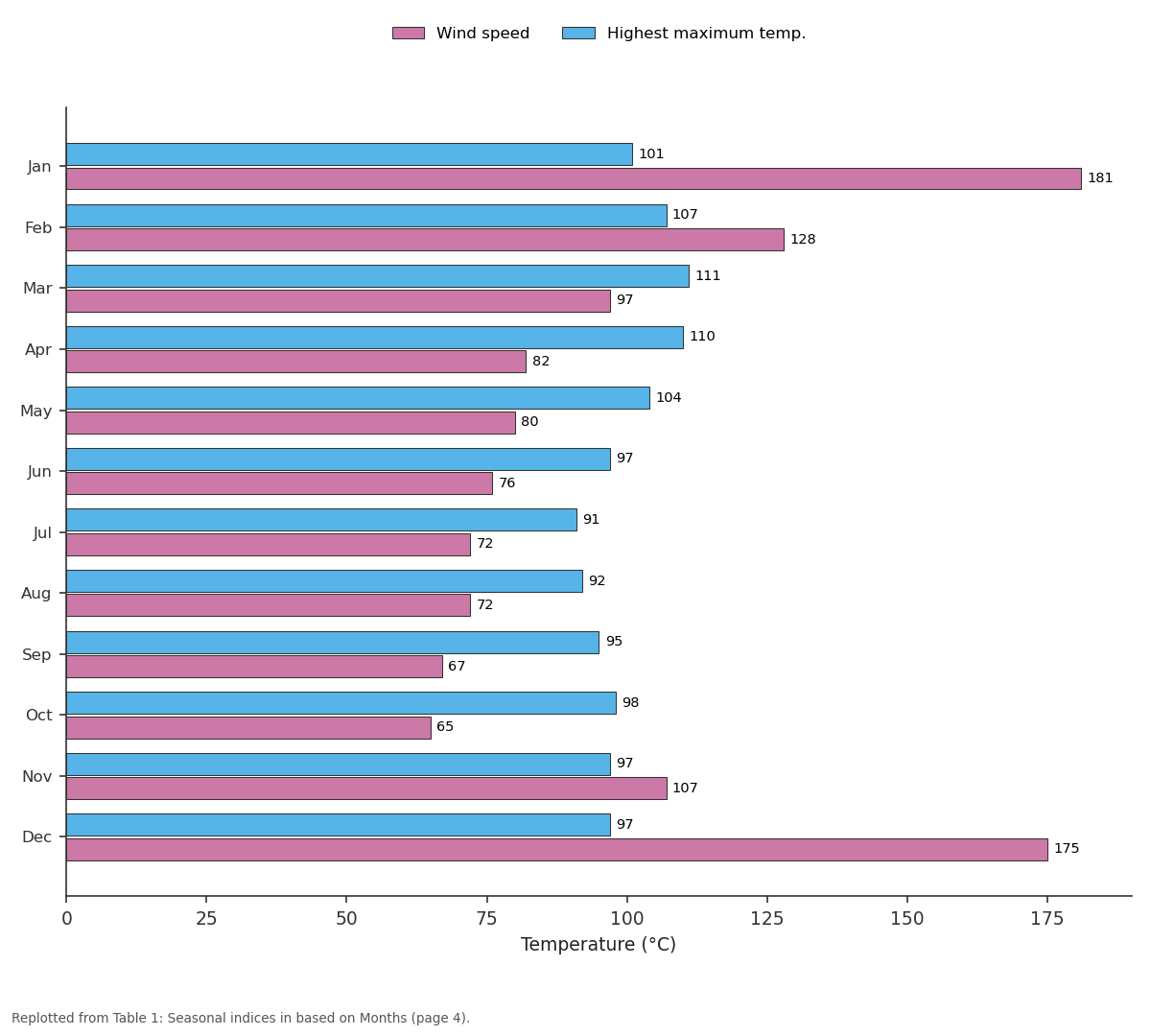
Wind speed and Highest maximum temp.: Jan vs Feb vs Mar vs Apr vs May
Replotted from Table 1 (page 4) of the original paper. Every bar is the paper's own table value.
View source evidence ↗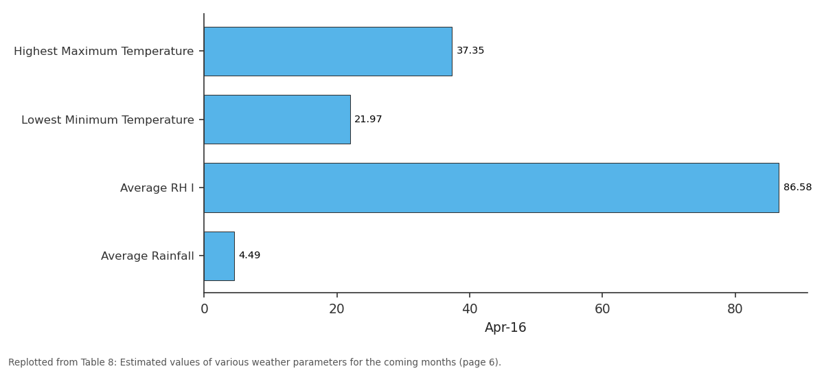
Apr-16: Highest Maximum... vs Lowest Minimum... vs Average RH I vs Average Rainfall
Replotted from Table 8 (page 6) of the original paper. Every bar is the paper's own table value.
View source evidence ↗Figures & tables
From the original paper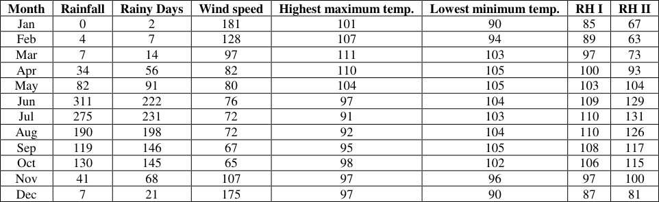 Table 1
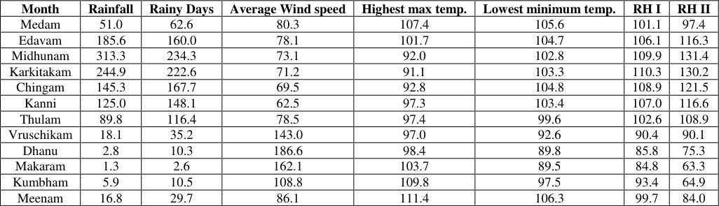 Table 2
 Table 3
 Table 4
 Table 5
 Table 6
 Table 7
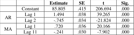 Table 8
 Table 9
 Table 10
 Table 11
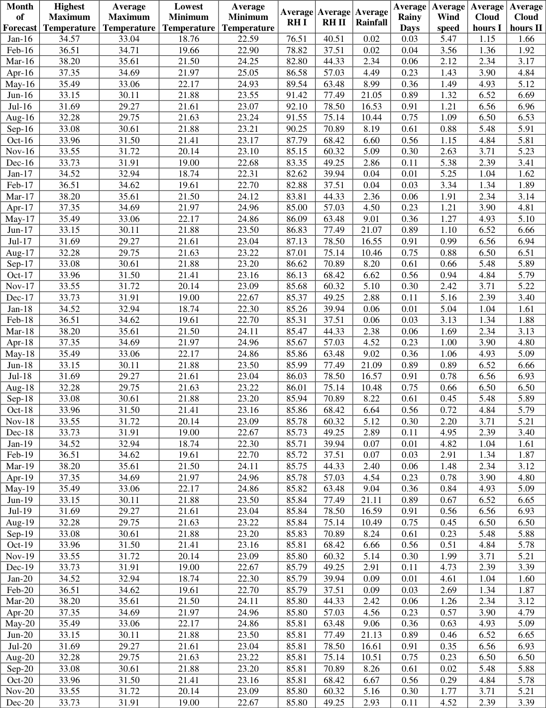 Table 8
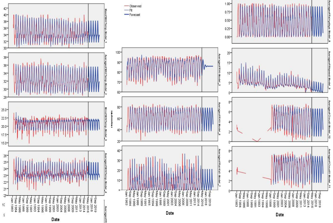 Figure 1
Introduction
Climate change and variability in recent decades are subjects of worldwide discussion as the weather related disasters viz., droughts, floods, ice storms, dust storms, hailstorms, landslides, heat and cold waves and thunder storms are not uncommon over one or another region of the world. Warming of the climate system is unequivocal. The atmosphere and ocean have warmed, the amounts of snow and ice have diminished and sea level has risen (IPCC, 2014) [7] . The range of temperature increase by end of the 21st century was projected to be between 1.1 to 6.4 °C across all scenarios. The report points out that if the temperature increases beyond 2.5 °C, then 20 to 30 per cent of known animal and plant species would be at increased risk of extinction. If the global average temperature increase exceeded 3.5 °C, models suggested that there would be extinctions of 40 to 70 per cent of known species (IPCC, 2014) [7] . India is one of the 27 Countries identified as most vulnerable to the impact of global warming. Lal et al., (1995) [17] predicted an increase in annual mean maximum and minimum surface air temperatures of 0.7 °C and 1.0 °C over land in the 2040s with respect to the 1980s. Lonergan (1998) [19] estimates that India's climate could become warmer under conditions of increased atmospheric carbon dioxide. The average temperature change is predicted to be in the range of 2.33 °C to 4.78 °C with doubling in CO2 concentrations. Lal et al., (2001) [18] , Kumar and Ashrit (2001) [16] , Kumar et al., (2002 and 2003) also predicted the temperature and rainfall trends over India under varied CO2 levels. Guhathakurta and Rajeevan (2007) observed decreasing trend in almost all subdivisions except for subdivisions Himachal Pradesh, Jharkhand and Nagaland, Manipur, Mizoram and Tripura during winter. Annual rainfall showed significant decreasing trend over Chhattisgarh, Jharkhand and Kerala. During southwest monsoon, Jharkhand, Chhattisgarh and Kerala showed significant decreasing trend in rainfall. Ramesh and Goswami (2007) [9,23] observed that decreasing trends in both early and late monsoon rainfall and number of rainy days for the period of 1951-2003, implying a shorter monsoon over India. Guhathakurta et al., (2011) [5] have studied the changes in the frequency of rainy days, rain days as well as heavy rainfall days using the daily rainfall data for the period 1901-2005 all over India. It is a fact that climate change is real and is happening across the world in different magnitudes.
Thrissur is the cultural capital of Kerala and the fourth largest city in the God's Own Country (Kerala State, India), which lies between North Latitudes 10° 10' 22" and 10° 46' 54" and East Longitudes 75° 57' 20" and 76° 54' 23". The climate of Thrissur is typical to the climate of Kerala i.e., Tropical monsoon (humid) type. The district is characterized by dry weather during summer months (March-May) with intermittent summer showers, blessed with two rainy seasons ie., southwest monsoon (June-September) and post monsoon (October -November) and pleasant winter months (December -February). The district is blessed with pleasant and periodic wind from November fortnight to February fortnight, known as the vrischika kaattu (the wind blowing during the local calendar Vrischikam though Makaram). The wind is characterised with heavy speed and having no moisture content as it passes through the Palakkad Gap of the Western Ghats and subsequently gains momentum. The district has a tropical humid climate with an oppressive hot season and plentiful of seasonal rainfall. Studies indicate that the State of Kerala is warming over a period of time. The India Meteorological Department has reported that the mean maximum temperature over the State has increased by 0.8 °C, mean minimum temperature by 0.2 °C and the average temperature by 0.5 °C between 1961 to 2003. Gopakumar (2017) [3] has reported that the mean annual temperature across the State of Kerala has increased by 0.65 °C (@0.011 °C/year) over a period time from 1956 to 2014. The increase in maximum temperature was 0.99 °C (@0.0169 °C/year) while that of minimum temperature was 0.31 °C(@0.0053 °C/year) during the same period (1956 to 2014). He has further reported that the rate of increase in temperature is high across the coastal belt when compared to mid and high range areas in the State. Further, the rate of increase in temperature was high during the post monsoon (0.76 °C over a period of six decades since 1956) followed by monsoon (increase of 0.732 °C over a period of six decades since 1956). Annual rainfall across the State of Kerala is showing a declining trend since last six decades. The decline in southwest monsoon rainfall is conspicuous. Soman et al., (1988) [25] reported that rainfall in Kerala showed significantly decreasing trend. Krishnakumar et al., (2007) [14] have reported that the rainfall in June and July was declining while increasing in August and September across the State of Kerala after analyzing the rainfall data of the State. Krishnakumar et al., (2009) [11,12] studied the temporal variation in monthly, seasonal and annual rainfall over Kerala during the period from 1871 to 2005 and reported significant decrease in southwest monsoon rainfall and increase in post-monsoon rainfall. Important aspect of the rainfall trend across the State of Kerala in the twentieth century was the significant decrease in the southwest monsoon rainfall and increase in post monsoon rainfall (Krishnakumar et al., 2009) [11,12] . There were large intra-regional differences in the trends in different seasons and local changes were found different from the large spatial scale averages in Kerala (Pal and Al-Tabba, 2009) [21] . Winter and autumn extreme rainfall were found to be having an increasing tendency with statistically significant changes in some regions indicating more occurrences of winter and autumn flood. Pillai et al. (2009) [22] analysed the trend of rainfall and the number of rainy days over 25 years and estimated regression models for Vellayani, Thiruvananthapuram. Unnikrishnan and Ajitha (2009) [26] developed a time series model for forecasting the onset of monsoon in Kerala using the data from 1870 to 2009. Gopakumar (2011) [11] revealed that the southwest monsoon rainfall in Kerala has been declining while increasing in post monsoon season. The annual rainfall exhibited a cyclic trend of 40-60 years, with a significant decline in recent decades and the moisture index across the State of Kerala indicate that the State was moving from wetness to dryness within the humid climate. SARIMA models are the most general forecasting models with high degree of accuracy. Considering the importance and unavoidable role of seasons in Kerala, time series models were developed using Seasonal Auto Regressive Integrated Moving Average (SARIMA) for forecasting monthly parameters for the Thrissur District. No previous attempts were seen to analyse the rainfall and temperature trends in the District using SARIMA model. Hence, an attempt has been made in the present paper to analyse the rainfall and temperature trends for the Thrissur District of Kerala using the SARIMA model.
Materials and methods
The present investigation was carried out at the Department of Statistics, Farook College during the period from 2012-2017. The study analysed the maximum temperature (°C), minimum temperature (°C), humidity at 7am and 2pm, cloud hours at 7am and 2pm, total rainfall (mm), number of rainy days and wind speed (km/hr.) trends for the Thrissur District of Kerala State, India. Daily weather data recorded at the Principal Agrometeorological Observatory at the Main Campus of the Kerala Agricultural University and maintained by the Department of Agricultural Meteorology, College of Horticulture, Kerala Agricultural University, Vellanikkara were collected for the period from 1983 to 2015. Monthly means were worked out using the daily data. An attempt has been made to develop new statistical tools for forecasting weather of Thrissur District. The main items of observations include maximum and minimum temperature, average/mean temperature and rainfall. Classical time series decomposition analysis was performed (Anderson, 1971) [1] for each of the weather parameters under study. Through this approach time series data were decomposed to identify four basic components, viz., the trend, seasonal fluctuations and cyclic variations and irregular. The multiplicative model of decomposition of the form Y = T*S*C*I, where Y denote the value corresponding to the dependent variable, S the seasonal component, C the cyclical part and I the irregular random component was used for the analysis. Box and Jenkins method is applied to fit forecasting models. This can apply only to stationary time series data. A time series is stationary on the space Rh+1 if the distribution of the vector of observations (Xt, Xt+1, Xt+2,…, Xt+h) is independent of t, h N. Many time series in real life are not stationary. A non-stationary sequence has to be transformed to a stationary sequence before attempting to apply a model for the same. A time series Xt is said to be an ARIMA (p,d,q) process if there exists polynomials and of degrees p and q respectively and a white noise series Zt such that (B)dXt = (B)Zt under the assumption that the time series dXt is stationary on the underlying probability space, where B denote the back shift operator B(Xt) =Xt-1. When d=0,Xt= [(B)/(B)]Zt , is a stationary ARMA(p,q) process and in this case all the zeroes of the polynomial (z) lie outside the unit circle |z| < 1. When it has one or more values equal to one but no value inside the unit circle, it is nonstationary but integrated. In this case the time series is an ARIMA process. In general when the function [(B)/(B)] is well defined and analytic in the region {zC | (z)0}, if has no roots on the circle {z | |z|=1}. Since it has p different roots there is an annulus {z/r<|z|<R} with r<1<R on which it has no root. On this annulus [(B)/(B) is analytic and it has a Laurent's series expansion (z)= jB j This series is uniformly and absolutely convergent on every compact subset of the annulus and the coefficients are uniquely determined by the value of Xt on the annulus. Hence the random variables Xt and Zt are defined on a probability space (U,P) and satisfying (B)dXt = (B)Zt for almost every Then the equation (B)dXt = (B)Zt takes the form XtXt-1Xt-2+...pXt-p + ZtZt-1Zt-2 +...+qZt-q For a stationary time series, the auto covariance and auto correlation at a lag kZ are defined by X(k) = cov(Xt+k, Xt) and X(k)) =(Xt+k, Xt) = X(k))/ X(0)), where X(0)= Var(Xt) and X(0) = 1. The partial auto correlation at a lag k is defined as the correlation between Xk -k-1(Xk) and X0 -k-1(X0), where k is the projection of the vector yRk on the subspace spanned by (X1,X2,…Xk) in Rk which is a linear combination y=bjxj such that ||y-y^|| is minimal. This is the correlation due to intermediate values X1,X2,…Xk-1 removed.
Seasonal ARIMA Modeling
Identification of relevant models and inclusion of suitable seasonal variables are necessary for seasonal modeling and their applications. The Seasonal ARIMA, ARIMA (p,d,q) (P,D,Q)s are defined by seven parameters. The seasonal part of an ARIMA model has the same structure as the nonseasonal part. It may have an AR factor, an MA factor and/or an order of differencing. In the seasonal part of the model, all of these factors operate across multiples of lag's' (the number of periods in a season). A seasonal ARIMA model is classified as an ARIMA (p,d,q) (P,D,Q)s model, where, P is the number of seasonal autoregressive (SAR) terms, D is the number of seasonal differences, Q is the number of seasonal moving average (SMA) terms. A general AR model with P SAR parameters is given by Yt = ∑ αisYt-is I =1 to p. Where Y t-sis of order s, Y t-2s is of order 2s and Y t-ps, is of order ps. A model with one SAR parameter is written as Yt s Yt-s e t Seasonal Moving Average (SMA) models are built with seasonal moving average (SMA) parameters, and the general SMA model with Q parameters is given by: Y t ∑is Yt-is et The general mixed SAR and SMA model is given by Yt = ∑ αisYt-is ∑is Yt-is et In identifying a seasonal model, the first step is to determine whether or not a seasonal difference is needed, in addition to or perhaps instead of a non-seasonal difference. By looking at the time series plots correlogram for all possible combinations of 0 or 1 non seasonal differences and 0 or 1 seasonal differences, the differences can be fixed. It is not good to use more than one seasonal and more than two non-seasonal differences. The signature of pure SAR or pure SMA behavior is similar to the signature of pure AR or pure MA behaviour, except that the pattern appears across multiples of lag's' in the ACF and PACF. For example, a pure SAR (1) process has spikes in the ACF at lags s, 2s, 3s, etc., while the PACF cuts off after lag s. Conversely, a pure SMA (1) process has spikes in the PACF at lags s, 2s, 3s, etc., while the ACF cuts off after lag s. An SAR signature usually occurs when the autocorrelation at the seasonal period is positive, whereas an SMA signature usually occurs when the seasonal autocorrelation is negative. If the autocorrelation at the seasonal period is positive, it is good to add one SAR term to the model. If the autocorrelation at the seasonal period is negative, it is better to add an SMA term to the model. It is not a good practice to mix with SAR and SMA terms in the same model. Usually an SAR (1) or SMA (1) term is sufficient. Although a seasonal ARIMA model seems to have only a few parameters, back forecasting requires the estimation of one or two seasons' worth of implicit parameters to initialize it. Therefore, it should have at least 4 or 5 seasons of data to fit a seasonal ARIMA model. Probably the most commonly used seasonal ARIMA model is the (0, 1, 1)×(0, 1, 1) model i.e., a MA(1) * SMA(1) model with both seasonal and a non-seasonal difference. This is essentially a "seasonal exponential smoothing" model. When seasonal ARIMA models are fitted to lag data, they are capable of tracking a multiplicative seasonal pattern. The best model is selected by using the diagnostic such as Coefficient of determination (R [2] used SARIMA time series modelling to fit the monthly average maximum and minimum temperature data sets collected at Giridih, India for the years 1990-2011. Goswami et al. (2017) [9,23] studied monthly temperature record in the Dibrugarh region using the Box-Jenkins (SARIMA) methodology. The analysis results revealed that the models' are adequately fitted to the historical data. Inderjeet Kaushik1 and Sabita Madhvi Singh (2008) observed Seasonal ARIMA models can predict minimum and maximum temperature with good accuracy as statistics of models indicate. G. Sathish et al. 2017 [24] used SARIMA model and found to be most suitable for forecasting total monthly rainfall over the Gangetic West Bengal. This model was considered appropriate to forecast the monthly rainfall for the next ten years in the Gangetic West Bengal region to assist policy makers to establish priorities for water demand, storage, distribution and disaster management. The real power and attractiveness of this method is that it can handle complex patterns using a relatively well specified set of rules. The Box-Jenkins methodology of forecasting is different from most methods because it does not assume any particular pattern in the historical data of the series to be forecasted. It uses an iterative approach to identify a possible model from a general class of models. The chosen model is then checked against the historical data to see whether it accurately describes the series. The model fits well if the residuals are generally small, randomly distributed and contain no useful information. If the specified model is not satisfactory, the process is repeated using a new model designed to improve on the original one. This iterative procedure continues until a satisfactory model is found.
Results and discussion
Seasonal indices were worked out for each parameters assuming multiplicative model of decomposition given by Yt = T X S X C X I, where T denote the general long term behavior of the series known as Trend, S denote the seasonality index, C denote the cyclic behavior of the time series and I the irregular random component of the series. The irregular part is identified by removing the trend, seasonality and cyclical parts. They are short term fluctuations on account of climatic deviations. In the case of evening relative humidity (RHII), SARIMA (0, 0, 1) (0, 1, 1)12 was the best model. The model is having an R 2 of 0.898 indicating that 89.8 percentage of variation in the data could be explained by the model and the MAPE was 6.895 percentage and RMSE was 4.726. The estimates of the parameters are given in Table 9.
| — | — | Estimate | SE | t | Sig. |
|---|---|---|---|---|---|
| MA | Lag 1 | -.210 | .050 | -4.202 | .000 |
| MA, Seasonal | Lag 1 | .916 | .034 | 26.740 | .000 |
Table text extracted from the original PDF; superscript letters are shown inline. The original table image is below.
View original table image
Conclusion
An attempt has been made to develop new statistical tools for forecasting weather in Thrissur District using SARIMA. Good fits were obtained for maximum temperature, minimum temperature, wind speed, measurements of Relative humidity at 7 am and 2pm and Average cloud hours with small MAPE and high R 2 value. In the case of rainfall and rainy days, the models were identified with a much higher MAPE and low R 2 values due to the high fluctuations in the data.
Figures and tables from the paper
| Month | Rainfall | Rainy Days | Wind speed | Highest maximum temp. | Lowest minimum temp. | RH I | RH II |
|---|---|---|---|---|---|---|---|
| Jan | 0 | 2 | 181 | 101 | 90 | 85 | 67 |
| Feb | 4 | 7 | 128 | 107 | 94 | 89 | 63 |
| Mar | 7 | 14 | 97 | 111 | 103 | 97 | 73 |
| Apr | 34 | 56 | 82 | 110 | 105 | 100 | 93 |
| May | 82 | 91 | 80 | 104 | 105 | 103 | 104 |
| Jun | 311 | 222 | 76 | 97 | 104 | 109 | 129 |
| Jul | 275 | 231 | 72 | 91 | 103 | 110 | 131 |
| Aug | 190 | 198 | 72 | 92 | 104 | 110 | 126 |
| Sep | 119 | 146 | 67 | 95 | 105 | 108 | 117 |
| Oct | 130 | 145 | 65 | 98 | 102 | 106 | 115 |
| Nov | 41 | 68 | 107 | 97 | 96 | 97 | 100 |
| Dec | 7 | 21 | 175 | 97 | 90 | 87 | 81 |
Table text extracted from the original PDF; superscript letters are shown inline. The original table image is below.
View original table image
| Month | Rainfall | Rainy Days | Average Wind speed | Highest max temp. | Lowest minimum temp. | RH I | RH II |
|---|---|---|---|---|---|---|---|
| Medam | 51.0 | 62.6 | 80.3 | 107.4 | 105.6 | 101.1 | 97.4 |
| Edavam | 185.6 | 160.0 | 78.1 | 101.7 | 104.7 | 106.1 | 116.3 |
| Midhunam | 313.3 | 234.3 | 73.1 | 92.0 | 102.8 | 109.9 | 131.4 |
| Karkitakam | 244.9 | 222.6 | 71.2 | 91.1 | 103.3 | 110.3 | 130.2 |
| Chingam | 145.3 | 167.7 | 69.5 | 92.8 | 104.8 | 108.9 | 121.5 |
| Kanni | 125.0 | 148.1 | 62.5 | 97.3 | 103.4 | 107.0 | 116.6 |
| Thulam | 89.8 | 116.4 | 78.5 | 97.4 | 99.6 | 102.6 | 108.9 |
| Vruschikam | 18.1 | 35.2 | 143.0 | 97.0 | 92.6 | 90.4 | 90.1 |
| Dhanu | 2.8 | 10.3 | 186.6 | 98.4 | 89.8 | 85.8 | 75.3 |
| Makaram | 1.3 | 2.6 | 162.1 | 103.7 | 89.5 | 84.8 | 63.3 |
| Kumbham | 5.9 | 10.5 | 108.8 | 109.8 | 97.5 | 93.4 | 64.9 |
| Meenam | 16.8 | 29.7 | 86.1 | 111.4 | 106.3 | 99.7 | 84.0 |
Table text extracted from the original PDF; superscript letters are shown inline. The original table image is below.
View original table image
| — | — | Estimate | SE | t | Sig. |
|---|---|---|---|---|---|
| MA | Lag 1 | -.220 | .051 | -4.348 | .000 |
| MA | Lag 2 | -.184 | .050 | -3.664 | .000 |
| MA, Seasonal | Lag 1 | .862 | .033 | 25.997 | .000 |
Table text extracted from the original PDF; superscript letters are shown inline. The original table image is below.
View original table image
| — | — | Estimate | SE | t | Sig. |
|---|---|---|---|---|---|
| MA | Lag 2 | -.129 | .050 | -2.549 | .011 |
| MA, Seasonal | Lag 1 | .933 | .039 | 24.036 | .000 |
Table text extracted from the original PDF; superscript letters are shown inline. The original table image is below.
View original table image
| — | — | Estimate | SE | t | Sig. |
|---|---|---|---|---|---|
| AR | Lag 1 | .205 | .050 | 4.087 | .000 |
| MA, Seasonal | Lag 1 | .932 | .035 | 26.544 | .000 |
Table text extracted from the original PDF; superscript letters are shown inline. The original table image is below.
View original table image
| — | — | Estimate | SE | t | Sig. |
|---|---|---|---|---|---|
| MA | Lag 1 | .657 | .039 | 16.778 | .000 |
| MA, Seasonal | Lag 1 | .841 | .034 | 24.747 | .000 |
Table text extracted from the original PDF; superscript letters are shown inline. The original table image is below.
View original table image
| — | — | — | Estimate | — | — | SE | — | — | t | — | Sig. | — |
|---|---|---|---|---|---|---|---|---|---|---|---|---|
| Constant | 85.805 | .415 | 206.694 | .000 | ||||||||
| AR | Lag 1 | 1.494 | .038 | 39.265 | .000 | |||||||
| Lag 2 | -.745 | .034 | -21.824 | .000 | ||||||||
| MA | Lag 1 | .720 | .036 | 20.166 | .000 | |||||||
| Lag 11 | -.241 | .030 | -7.902 | .000 |
Table text extracted from the original PDF; superscript letters are shown inline. The original table image is below.
View original table image
| — | — | Estimate | SE | t | Sig. |
|---|---|---|---|---|---|
| MA | Lag 1 | .191 | .071 | 2.699 | .008 |
| MA, Seasonal | Lag 1 | .770 | .054 | 14.134 | .000 |
Table text extracted from the original PDF; superscript letters are shown inline. The original table image is below.
View original table image
| — | — | Estimate | SE | t | Sig. |
|---|---|---|---|---|---|
| AR | Lag 1 | .917 | .066 | 13.896 | .000 |
| MA | Lag 1 | .792 | .098 | 8.079 | .000 |
| MA, Seasonal | Lag 1 | .835 | .060 | 13.849 | .000 |
Table text extracted from the original PDF; superscript letters are shown inline. The original table image is below.
View original table image
| Month of Forecast | Highest Maximum Temperature | Average Maximum Temperature | Lowest Minimum Temperature | Average Minimum Temperature | Average RH I | Average RH II | Average Rainfall | Average Rainy Days | Average Wind speed | Average Cloud hours I | Average Cloud hours II |
|---|---|---|---|---|---|---|---|---|---|---|---|
| Jan-16 | 34.57 | 33.04 | 18.76 | 22.59 | 76.51 | 40.51 | 0.02 | 0.03 | 5.47 | 1.15 | 1.66 |
| Feb-16 | 36.51 | 34.71 | 19.66 | 22.90 | 78.82 | 37.51 | 0.02 | 0.04 | 3.56 | 1.36 | 1.92 |
| Mar-16 | 38.20 | 35.61 | 21.50 | 24.25 | 82.80 | 44.33 | 2.34 | 0.06 | 2.12 | 2.34 | 3.17 |
| Apr-16 | 37.35 | 34.69 | 21.97 | 25.05 | 86.58 | 57.03 | 4.49 | 0.23 | 1.43 | 3.90 | 4.84 |
| May-16 | 35.49 | 33.06 | 22.17 | 24.93 | 89.54 | 63.48 | 8.99 | 0.36 | 1.49 | 4.93 | 5.12 |
| Jun-16 | 33.15 | 30.11 | 21.88 | 23.55 | 91.42 | 77.49 | 21.05 | 0.89 | 1.32 | 6.52 | 6.69 |
| Jul-16 | 31.69 | 29.27 | 21.61 | 23.07 | 92.10 | 78.50 | 16.53 | 0.91 | 1.21 | 6.56 | 6.96 |
| Aug-16 | 32.28 | 29.75 | 21.63 | 23.24 | 91.55 | 75.14 | 10.44 | 0.75 | 1.09 | 6.50 | 6.53 |
| Sep-16 | 33.08 | 30.61 | 21.88 | 23.21 | 90.25 | 70.89 | 8.19 | 0.61 | 0.88 | 5.48 | 5.91 |
| Oct-16 | 33.96 | 31.50 | 21.41 | 23.17 | 87.79 | 68.42 | 6.60 | 0.56 | 1.15 | 4.84 | 5.81 |
| Nov-16 | 33.55 | 31.72 | 20.14 | 23.10 | 85.15 | 60.32 | 5.09 | 0.30 | 2.63 | 3.71 | 5.23 |
| Dec-16 | 33.73 | 31.91 | 19.00 | 22.68 | 83.35 | 49.25 | 2.86 | 0.11 | 5.38 | 2.39 | 3.41 |
| Jan-17 | 34.52 | 32.94 | 18.74 | 22.31 | 82.62 | 39.94 | 0.04 | 0.01 | 5.25 | 1.04 | 1.62 |
| Feb-17 | 36.51 | 34.62 | 19.61 | 22.70 | 82.88 | 37.51 | 0.04 | 0.03 | 3.34 | 1.34 | 1.89 |
| Mar-17 | 38.20 | 35.61 | 21.50 | 24.12 | 83.81 | 44.33 | 2.36 | 0.06 | 1.91 | 2.34 | 3.14 |
| Apr-17 | 37.35 | 34.69 | 21.97 | 24.96 | 85.00 | 57.03 | 4.50 | 0.23 | 1.21 | 3.90 | 4.81 |
| May-17 | 35.49 | 33.06 | 22.17 | 24.86 | 86.09 | 63.48 | 9.01 | 0.36 | 1.27 | 4.93 | 5.10 |
| Jun-17 | 33.15 | 30.11 | 21.88 | 23.50 | 86.83 | 77.49 | 21.07 | 0.89 | 1.10 | 6.52 | 6.66 |
| Jul-17 | 31.69 | 29.27 | 21.61 | 23.04 | 87.13 | 78.50 | 16.55 | 0.91 | 0.99 | 6.56 | 6.94 |
| Aug-17 | 32.28 | 29.75 | 21.63 | 23.22 | 87.01 | 75.14 | 10.46 | 0.75 | 0.88 | 6.50 | 6.51 |
| Sep-17 | 33.08 | 30.61 | 21.88 | 23.20 | 86.62 | 70.89 | 8.20 | 0.61 | 0.66 | 5.48 | 5.89 |
| Oct-17 | 33.96 | 31.50 | 21.41 | 23.16 | 86.13 | 68.42 | 6.62 | 0.56 | 0.94 | 4.84 | 5.79 |
| Nov-17 | 33.55 | 31.72 | 20.14 | 23.09 | 85.68 | 60.32 | 5.10 | 0.30 | 2.42 | 3.71 | 5.22 |
| Dec-17 | 33.73 | 31.91 | 19.00 | 22.67 | 85.37 | 49.25 | 2.88 | 0.11 | 5.16 | 2.39 | 3.40 |
| Jan-18 | 34.52 | 32.94 | 18.74 | 22.30 | 85.26 | 39.94 | 0.06 | 0.01 | 5.04 | 1.04 | 1.61 |
| Feb-18 | 36.51 | 34.62 | 19.61 | 22.70 | 85.31 | 37.51 | 0.06 | 0.03 | 3.13 | 1.34 | 1.88 |
| Mar-18 | 38.20 | 35.61 | 21.50 | 24.11 | 85.47 | 44.33 | 2.38 | 0.06 | 1.69 | 2.34 | 3.13 |
| Apr-18 | 37.35 | 34.69 | 21.97 | 24.96 | 85.67 | 57.03 | 4.52 | 0.23 | 1.00 | 3.90 | 4.80 |
| May-18 | 35.49 | 33.06 | 22.17 | 24.86 | 85.86 | 63.48 | 9.02 | 0.36 | 1.06 | 4.93 | 5.09 |
| Jun-18 | 33.15 | 30.11 | 21.88 | 23.50 | 85.99 | 77.49 | 21.09 | 0.89 | 0.89 | 6.52 | 6.66 |
| Jul-18 | 31.69 | 29.27 | 21.61 | 23.04 | 86.03 | 78.50 | 16.57 | 0.91 | 0.78 | 6.56 | 6.93 |
| Aug-18 | 32.28 | 29.75 | 21.63 | 23.22 | 86.01 | 75.14 | 10.48 | 0.75 | 0.66 | 6.50 | 6.50 |
| Sep-18 | 33.08 | 30.61 | 21.88 | 23.20 | 85.94 | 70.89 | 8.22 | 0.61 | 0.45 | 5.48 | 5.89 |
| Oct-18 | 33.96 | 31.50 | 21.41 | 23.16 | 85.86 | 68.42 | 6.64 | 0.56 | 0.72 | 4.84 | 5.79 |
| Nov-18 | 33.55 | 31.72 | 20.14 | 23.09 | 85.78 | 60.32 | 5.12 | 0.30 | 2.20 | 3.71 | 5.21 |
| Dec-18 | 33.73 | 31.91 | 19.00 | 22.67 | 85.73 | 49.25 | 2.89 | 0.11 | 4.95 | 2.39 | 3.40 |
| Jan-19 | 34.52 | 32.94 | 18.74 | 22.30 | 85.71 | 39.94 | 0.07 | 0.01 | 4.82 | 1.04 | 1.61 |
| Feb-19 | 36.51 | 34.62 | 19.61 | 22.70 | 85.72 | 37.51 | 0.07 | 0.03 | 2.91 | 1.34 | 1.87 |
| Mar-19 | 38.20 | 35.61 | 21.50 | 24.11 | 85.75 | 44.33 | 2.40 | 0.06 | 1.48 | 2.34 | 3.12 |
| Apr-19 | 37.35 | 34.69 | 21.97 | 24.96 | 85.78 | 57.03 | 4.54 | 0.23 | 0.78 | 3.90 | 4.80 |
| May-19 | 35.49 | 33.06 | 22.17 | 24.86 | 85.82 | 63.48 | 9.04 | 0.36 | 0.84 | 4.93 | 5.09 |
| Jun-19 | 33.15 | 30.11 | 21.88 | 23.50 | 85.84 | 77.49 | 21.11 | 0.89 | 0.67 | 6.52 | 6.65 |
| Jul-19 | 31.69 | 29.27 | 21.61 | 23.04 | 85.84 | 78.50 | 16.59 | 0.91 | 0.56 | 6.56 | 6.93 |
| Aug-19 | 32.28 | 29.75 | 21.63 | 23.22 | 85.84 | 75.14 | 10.49 | 0.75 | 0.45 | 6.50 | 6.50 |
| Sep-19 | 33.08 | 30.61 | 21.88 | 23.20 | 85.83 | 70.89 | 8.24 | 0.61 | 0.23 | 5.48 | 5.88 |
| Oct-19 | 33.96 | 31.50 | 21.41 | 23.16 | 85.81 | 68.42 | 6.66 | 0.56 | 0.51 | 4.84 | 5.78 |
| Nov-19 | 33.55 | 31.72 | 20.14 | 23.09 | 85.80 | 60.32 | 5.14 | 0.30 | 1.99 | 3.71 | 5.21 |
| Dec-19 | 33.73 | 31.91 | 19.00 | 22.67 | 85.79 | 49.25 | 2.91 | 0.11 | 4.73 | 2.39 | 3.39 |
| Jan-20 | 34.52 | 32.94 | 18.74 | 22.30 | 85.79 | 39.94 | 0.09 | 0.01 | 4.61 | 1.04 | 1.60 |
| Feb-20 | 36.51 | 34.62 | 19.61 | 22.70 | 85.79 | 37.51 | 0.09 | 0.03 | 2.69 | 1.34 | 1.87 |
| Mar-20 | 38.20 | 35.61 | 21.50 | 24.11 | 85.80 | 44.33 | 2.42 | 0.06 | 1.26 | 2.34 | 3.12 |
| Apr-20 | 37.35 | 34.69 | 21.97 | 24.96 | 85.80 | 57.03 | 4.56 | 0.23 | 0.57 | 3.90 | 4.79 |
| May-20 | 35.49 | 33.06 | 22.17 | 24.86 | 85.81 | 63.48 | 9.06 | 0.36 | 0.63 | 4.93 | 5.09 |
| Jun-20 | 33.15 | 30.11 | 21.88 | 23.50 | 85.81 | 77.49 | 21.13 | 0.89 | 0.46 | 6.52 | 6.65 |
| Jul-20 | 31.69 | 29.27 | 21.61 | 23.04 | 85.81 | 78.50 | 16.61 | 0.91 | 0.35 | 6.56 | 6.93 |
| Aug-20 | 32.28 | 29.75 | 21.63 | 23.22 | 85.81 | 75.14 | 10.51 | 0.75 | 0.23 | 6.50 | 6.50 |
| Sep-20 | 33.08 | 30.61 | 21.88 | 23.20 | 85.81 | 70.89 | 8.26 | 0.61 | 0.02 | 5.48 | 5.88 |
| Oct-20 | 33.96 | 31.50 | 21.41 | 23.16 | 85.81 | 68.42 | 6.67 | 0.56 | 0.29 | 4.84 | 5.78 |
| Nov-20 | 33.55 | 31.72 | 20.14 | 23.09 | 85.80 | 60.32 | 5.16 | 0.30 | 1.77 | 3.71 | 5.21 |
| Dec-20 | 33.73 | 31.91 | 19.00 | 22.67 | 85.80 | 49.25 | 2.93 | 0.11 | 4.52 | 2.39 | 3.39 |
Table text extracted from the original PDF; superscript letters are shown inline. The original table image is below.
View original table image
References
26 in the original paper- Anderson TW. The Statistical Analysis of Time Series. John Wiley and Sons, New York, 1971, 704.
- Enakshi Saha, Arnab Hazra, Pabitra Banik. SARIMA modelling of the monthly average maximum and minimum temperatures in the eastern plateau region of India, Mausam. 2016; 67(4):841-848.
- Gopakumar. Climate variability of Kerala: Recent trends. Paper presented at the Press club, Thrissur in connection with the World Water Day Celebration on 22.3.2017, 2017.
- Gopakumar CS. Impacts of Climate variability on Agriculture in Kerala, PhD Thesis, Cochin University of Science and Technology, Cochin, 2011; 22:286.
- Guhathakurta P, Sreejith OP, Menon PA. Impact of climate change on extreme rainfall events and flood risk in India J Earth Syst. Sci. 2011; 120(3):359-373.
- Inderjeet Kaushik1, Sabita Madhvi Singh. Seasonal ARIMA model for forecasting of Monthly rainfall and temperature, Journal of Environmental Research and Development. 2008; 3(2):506-514.
- Intergovernmental Panel of Climate Change. Climate Change 2014, Synthesis Report, Summary for Policy makers. http://www.ipcc.ch/pdf/assessmentreport/ar5/syr/AR5_SYR_FINAL_SPM.pdf, 2014.
- IPCC (Intergovernmental Panel for Climate Change). Climate Change 2007: The Physical Science Basis IPCC Working Group I, 2007.
- Goswami K, Hazarika J, Patowary AN. Monthly temperature prediction based on arima model: a case study in dibrugarh station of assam, india, International Journal of Advanced Research in Computer Science. 2017; 8(8):292-298.
- Kotteswaram Alvi, SMA. Secular trends and periodicities in rainfall at West Coast stations in India. Curr. Sci. 1969; 101:371-375.
- Krishnakumar KN, Rao GSLHVP, Gopakumar CS. Rainfall trends in twentieth century over Kerala, India. Atmospheric environment, 2009; 43:1940-1944.
- Krishnakumar KN, Rao GSLHVP, Gopakumar CS. Rainfall trends in twentieth century over Kerala, India. Atmos. Environ, 2009; 43:1940-1944.
- Krishnakumar KN, Rao GSLHVP, Gopakumar CS. Climate change at selected locations in the humid tropics. J Agrometeorol. 2008; 10(1):59-64.
- Krishnakumar KN, Rao GSLHVP, Gopakumar CS, Mohan HSR. Rainfall variability during southwest monsoon over Kerala (India): 1971-2005. Indian Journal of Polar Sciences, 2007; 1:81-87.
- Kumar KR, Kumar KK, Ashrit RG, Patwardhan SK, Pant GB. Climate change in India: Observation and Model Projections. Climate change and India: Issues, Concern and Opportunities (eds. Shukla, P.R., Sharma, K.S. and Ramana, P.V.). Tata McGraw-Hill Publishing Company Ltd. New Delhi, 2002, 24-75.
- Kumar KR, Ashrit RG. Regional Aspects of global climate change simulations: Validation and assessment of climate response over Indian monsoon region to transient increase of greenhouse gases and sulphate aerosols. Mausam, 2001; 52(1):229-244.
- Lal M, Cubasch U, Voss R, Waszkewitz J. Effect of transient increases in greenhouse gases and sulphate aerosols on monsoon climate. Curr. Sci. 1995; 69(9):752763.
- Lal M, Nozawa T, Emori S, Harasawa H, Takahashi K, Kimoto M, et al. Future climate change: Implications for Indian summer monsoon and its variability. Curr. Sci. 2001; 81:1196-1207.
- Lonergan S. Climate warming and India, In Measuring the Impact of Climate Change on Indian Agriculture, (eds. Dinar, A et al.,) Washington DC: World Bank Technical Paper No. 402, 1998.
- Naidu CV, Rao BRS, Rao DVB. Climatic trends and periodicities of annual rainfall over India. Meteorol. Appl., 1999; 6:395-404.
- Pal I, Al-Tabbaa A. Trends in seasonal precipitation extremes -An indicator of 'climate change' in Kerala. Indian J of Hydrology. 2009; 367(1-2):62-69.
- Pillai S, Ajithkumar CE, Liji EG, Preetha PS. Seasonal variability and trend in rainfall and temperature at Vellayani. In: Proc. of the National Seminar on Climate Change Adaptation Strategies in Agriculture and Allied Sectors, KAU, 2009, 32-38.
- Ramesh KV, Goswami P. Reduction in Spatial and Temporal Extent of Monsoon rainfall, Geophy Res Lett, 2007; 34, L23704 doi:10.1029/ 2007GL031613, 2007.
- Sathish G, Lakshmi Narasinhaiah P, Mahesh Babu, Samrat Laha and n. Bharath kumar, 2017. Time series analysis of monthly rainfall for gangetic west bengal using box jenkins sarima modeling, int. j curr. microbiol. app. Sci. 2017; 6(7):2603-2610.
- Soman MR, Krishnakumar K, Singh N. Decreasing trend in the rainfall of Kerala. Curr. Sci., 1988; 57:7-12.
- Unnikrishnan T, Ajitha TK. A Univariate Statistical approach to predict the onset of South West Monsoon in India. In: Proc. of the National Workshop on Climate and Development, 29 th June 2009, Vellayani, Trivandrum, 2009, 8-16.
Cited by 1
From OpenAlex, OpenCitations and reference lists read by Scinovex
- Statistical Modelling of Maximum and Minimum Temperature in Thiruvananthapuram District ↗
G Dhanya · International Journal for Research in Applied Science and Engineering Technology · 2019
Time series analysis on maximum and minimum temperature using ARIMA model was done separately with the monthly mean temperature for the period from 1985-86 to 2013-14.The best fit ARIMA model for forecasting was selected based on different selection criteria viz., AIC (Akaike Information Criterion), BIC (Bayesian Information Criterion), Hannan-Quinn etc.In case of maximum temperature, ARIMA (101) (111) was the best…
❝ 0PDF