
Research article · 2017 · Full text
International Journal of Statistics and Applied MathematicsWhy so negative on negative volatilities
Volume 2(5) · Pages 116–124
Research areasStochastic processes and financial applicationsEconomic theories and models
Abstract
Author-writtenMost financial models are mathematically rigorously formulated using continuous time. However, asset prices in reality appear in discrete time intervals. Hence, there is the need to discretize financial models. During the process of discretization, stochastic volatilities can get negative. The typical way of dealing with this problem is setting these negative volatilities to zero. This is arbitrary and conceptually inconsistent. We argue that it is a better solution to accept negative volatilities and integrate them into the model. In this paper, we define negative volatilities, give examples how they occur in financial modeling and derive a mathematical theory of negative volatilities.
Summary
Source-checkedPlain-language reading of the full paper, prepared with AI and checked against the text. Each point links to the authors' own words.
Why it matters
- Financial models are typically designed for continuous time, but because real asset prices occur in discrete intervals, these models must be discretized. View evidence ↗
- Discretizing models can result in negative stochastic volatilities; the common practice of resetting these values to zero is viewed by the authors as arbitrary and inconsistent. View evidence ↗
- Volatility serves as a measure of security risk, representing the rate at which a security's price increases or decreases. View evidence ↗
The question
- The authors aim to define negative volatilities, demonstrate how they arise in financial modeling, and develop a mathematical theory to integrate them into models rather than ignoring them. View evidence ↗
What they did
- Standard volatility is typically calculated as the standard deviation of logarithmic returns over a specific time period. View evidence ↗
- The authors introduce 'nonstandard volatility,' which uses the average absolute deviation from the mean instead of the standard deviation. View evidence ↗
What they found
- In the discretized Heston model, negative volatilities occur particularly when the mean reversion parameter is low, the volatility of volatility is high, and random drawings are extreme. View evidence ↗
- Analysis of Dow 30 stocks shows a high correlation between standard and nonstandard volatility, with a correlation coefficient R = 0.9678 and R² = 0.9366. View evidence ↗
- The authors found that standard volatility is always greater than or equal to nonstandard volatility because average absolute deviation is less than or equal to standard deviation. View evidence ↗
- The mathematical model for signed volatility (type 1) results in a value of 0 if the asset price remains constant. View evidence ↗
- The signed volatility of the first type is 0 when the asset price changes proportionally by a constant factor k. View evidence ↗
What it means
- The authors conclude that negative volatilities should be accepted and integrated into financial models rather than being arbitrarily set to zero. View evidence ↗
- The authors recommend that quantitative analysts use either negative volatilities or negative probabilities to address options with negative intrinsic values. View evidence ↗
Figures & tables
From the original paper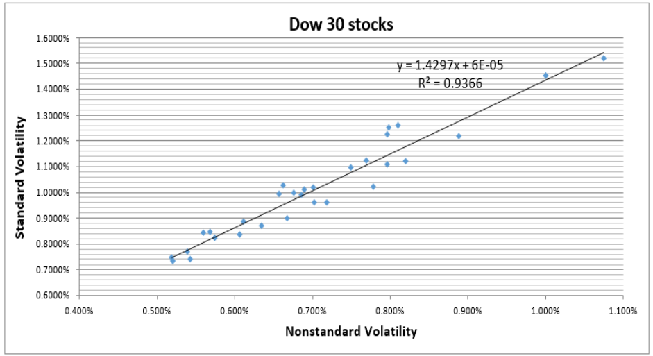 Figure 1
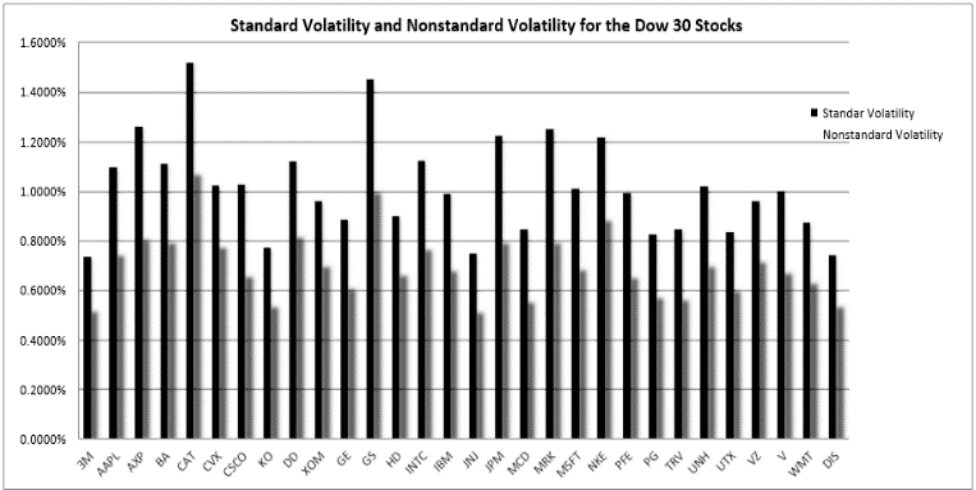 Figure 2
Introduction
New discoveries have always been met with skepticism and criticism. When negative numbers were introduced to Europe in books of Eastern mathematicians, critics dismissed their sensibility. European mathematicians such as Jean le Rondd' Alembert (1717-1783) or Augustus De Morgan (1806-1871) rejected negative numbers until the 18th century and referred to them as 'absurd' or 'meaningless' (see (Kline, 1980;Mattessich, 1998)) [5] . Likewise, irrational numbers and later imaginary numbers were firstly rejected. Today these concepts are accepted and applied in numerous scientific and practical fields, such as physics, chemistry, biology and finance. In addition, negative and above 1 probabilities were long assumed senseless. However, in the recent past they have gained acceptance and are applied in physics and finance (see (Mack, 2002;Haug, 2004;Sjöstrand, 2006;Kovner and Lublinsky, 2007;Venter, 2007;Burgin and Meissner 2012a, and 2012b) [3, 10, 6, 11, 1, 2] The rest of the paper is organized as follows. Section 2 defines volatility. Section 3 discusses volatilities in finance and analyses two popular financial models, in which discretization leads to negative volatilities. Section 4 introduces and studies nonstandard volatility. Section 5 derives a rigorous mathematical model for negative volatilities. Section 6 contains conclusions.
Definition of Volatility
Volatility is a rate at which the price of a security increases or decreases for a given set of returns. Volatility measures the risk of a security. It is used in option pricing formula to gauge the fluctuations in the returns of the underlying assets. Volatility indicates the pricing behavior of the security and providing estimation of the fluctuations that may happen in a short interval of time. Usually volatility is measured by calculating the standard deviation of the logarithmic returns over a given interval of time. It shows the range to which the price of a security may increase or decrease. For instance, annualized volatility σ is the standard deviation of the asset's yearly logarithmic returns. Thus, we have the following definition.
Definition 2.1. Volatility is the standard deviation of logarithmic price changes.
To construct a formula corresponding to this definition, we use the following notation. Let St be the price of an asset A, e.g. a stock price, at time t. Then the natural logarithmic price change from t to t+1 is ln(St+1/St) and we define the volatility σ of the price S as (1) In this formula, ln is the natural logarithm, n is the total number of prices, and S is the average of the logarithmic price changes, i. The advantage of using logarithmic price changes is that they are additive in time, whereas percentage changes are not (see (Meissner, 2014, chapter 1) for details).
There are two basic types of volatility historic volatility is derived from time series of past market prices; implied volatility is derived from the market price of a market traded derivative such as an option.
In turn, historic volatility is subdivided into the following classes: actual current volatility of an asset is defined for a specified interval of time, e.g., for one month or one year, based on real prices over this interval ending with the most recent price; actual historic volatility of an asset is also defined for a specified interval of time but ending with the price at a date in the past; realized volatility is calculated using the sum of squared returns divided by the number of observations; actual future volatility of an asset is defined for a specified interval of time, e.g., for one month or one year, based on real prices over this interval starting with the recent price and ending with the price at a future date, which is usually the expiry date of an option.
Implied volatility is also subdivided into several classes historical implied volatility of an asset refers to the implied volatility observed from historical prices of this asset; current implied volatility of an asset refers to the implied volatility derived from current prices of this asset; future implied volatility of an asset refers to the implied volatility developed using predictions of the future prices of this asset.
Examples of negative volatilities
Formula (1) implies that volatilities are always positive. However, there are several situations when negative volatilities emerge.
Negative volatilities in trading systems
In standard finance, asset prices S cannot be negative, therefore S 0. Hence from equations (1) and (2), it follows that volatility σ cannot be negative. This is intuitive, since volatility is the fluctuation intensity of a variable, which has a minimum of zero in the case when the variable is constant. However, in trading practice, especially in times of high volatility, option traders sometimes cannot pull their option positions fast enough out of the trading system. This can lead to arbitrage opportunities, i.e. option prices fall below the intrinsic value.1 This in turn implies negative implied volatility, which is used as input into an option pricing model such as the Black-Scholes-Merton model applied for deriving the option price. In today's trading environment, arbitrage opportunities only last milliseconds before they are realized by high-frequency traders.
Negative volatilities generated by discretization
Financial models are typically formulated in continuous time. However since in reality asset prices appear in discrete time units, there is a need to discretize continuous time models. In this process, often volatilities get negative2. We will show this with two popular models and argue that rather than arbitrarily setting negative volatilities to zero, it is more sensible to accept and work with negative volatilities. This is conceptually similar to accepting and applying imaginary numbers such as i2 = -1.
Discretization of Heston 1993 model
The seminal Heston 1993 model consists of three main equations. The first equation, the geometric Brownian motion of the stock price, is
Where S (t) : variable of interest, e.g. a stock price µ: (constant) expected growth rate of S σ(t) :expected volatility of S dz: standard Brownian motion, i.e. dz(t) = ε(t) , ε(t)i.i.d., is the variable which addsstochasticity. In particular ε(t) is a random drawing from a standardized normal distribution at time t, ε(t) = n~(0,1). ε can be computed with =normsinv (rand) in where a : mean reversion rate (gravity), i.e. degree with which σ at time t, σt, is pulled back to its long term mean mρ. 'a' is bounded in 0 ≤ a ≤ 1 (a > 1 would be 'overshooting the mean' and a < 0 would be 'mean-flight') mσ: long term mean of the σ ξ : (constant) volatility of the volatility σ Steven Heston in 1993 correlated equations ( 3) and ( 4) by correlating the Brownian motions dz1 and dz2 with the identity (5) where dz2(t) and dz3(t) are independent, and dz(t) and dz(t') are independent in time i.e. t ≠ t', and α is a correlation coefficient -1 ≤ α ≤ 1. Equation ( 5) is mathematically and computationally convenient. Indeed, if dz2 and dz3 are standard normal, it follows by construction that dz1 will also be standard normal for any value of -1 ≤ α ≤ 1. The model of equations ( 3) to ( 5) is formulated in continuous time. However, as mentioned, asset prices in reality appear in discrete time intervals. Hence, to apply the model to reality we need to discretize it. The discretized version of the Heston model is (3a) where ∆t can be any discrete time unit, e.g. a second, a day or a year. In empirical financial analyses, often end of day prices are used. In this case, ∆t is one day. Equation (4) discretizes changes to (4a) where Since in equations (3a) and (4a) the time units are discrete, i.e. ∆t, ∆z3 is now Hence in equation ( 5a) is (5a) Importantly, in the discrete model of equations (3a) to (5a), volatilities σ can get negative. This is especially the case when the mean reversion parameter 'a' is low, the volatility of volatility ξ is high and the random drawing ԑ is very high or very low. The negative values of volatility are typically considered undesired. For instance, Broadie and Kaya (2006) write: "To avoid the negative values for volatility and price, we set these to zero if we encounter negative values during the simulation". We argue that rather than arbitrarily and conceptually inconsistently setting the volatility to zero, to accept the negative volatilities and apply them to the model. In section 4 we derive a mathematical theory of negative volatility. We will now discuss a discretization of another model.
Discretization of the bounded Jacobi process
The bounded Jacobi process models a stochastic variable, which can be bounded. A popular variable, which is typically modeled by the Jacobi process, is the Pearson correlation coefficient ρ, which is bounded between -1 and +1. In continuous time we have where ρ : Pearson correlation coefficient, -1 ≤ ρ ≤ +1 a : mean reversion speed (gravity), i.e. degree with which the correlation at time t, ρt, is pulled back to its long term mean mρ. a can take the values 0 ≤ a ≤ 1. mρ: long term mean of the correlation ρ σρ: volatility of ρ h : upper boundary level, f : lower boundary level, i.e. h ≥ ρ ≥ f dz: standard Brownian motion, i.e. is i.i.d
With equation ( 6) the user can choose specific upper and lower boundaries. For correlation modeling in the Pearson framework, these boundaries are h = +1 and f = -1. In this case equation ( 6) reduces to (7) Equations ( 6) requires correlation values within a lower bound f and an upper bound h (otherwise the term cannot be evaluated). Equation ( 7) requires correlation values within the bounds -1 to +1
(otherwise, the term cannot be evaluated).Therefore
we have to introduce boundary conditions. These boundaries conditions for equation ( 6) are (8) for the lower bound f and ( 9)
for the higher bound h. Applying the boundary levels f = -1 and h = +1, we derive the boundary condition for equation ( 7) as (10) for the lower bound f and (11) for the higher bound h. The boundary conditions (8) to (11) are intuitive: The lower the volatility σ (or its square the variance rate σ2), and the higher the mean reversion rate 'a', the lower the fluctuation of ρ, guaranteeing that ρ stays within its boundaries. Discretizing equation (7), applying dρ = ρt+1 -ρt, we derive (12)
The boundary conditions (8) to (11) only guarantee that -1 ≤ρ≤ 1 for the continuous time model of equation (7). Even if the boundaries conditions (8) to (11) are satisfied, the discretized model of equation ( 12) can lead to values of ρ > 1 and ρ < -1.3 Importantly, if we model the volatility σρ of ρ with a stochastic process such as described by equation 4a, negative volatilities may occur. This will especially be case if the mean reversion rate 'a' is rather low, the volatility of volatility ξ is high and the random drawing ԑ is very high or very low. We argue that rather than setting these negative volatilities arbitrarily to zero, we should accept the negative volatilities and use them in the model. These would be financially, conceptually and mathematically rigorous and consistent.
A nonstandard model of volatility
To find a mathematically rigorous solution to the problem of negative volatilities, we introduce a nonstandard model of volatility and show that it is strongly correlated with the standard mathematical definition of volatility. This allows using the nonstandard volatility as the rate at which the price of a security increases or decreases for a given set of returns and as a measure of the risk of a security indicating the pricing behavior of the security and providing estimation of the fluctuations that may happen in a short period of time. While standard volatility is based on the formula of standard deviation, nonstandard volatility is based on the formula of average absolute deviation or absolute deviation from the mean, which is the sum of absolute values of the deviations divided by the number of observations. This gives us the following definition of nonstandard volatility. Here St is the price of an asset, e.g. a stock price, at time t, ln is the natural logarithm, the natural logarithmic price change from t to t+1 is ln(St+1/St), n is the total number of changes of prices and S̅ is the average of the logarithmic price changes, i.e. ( 14) Empirical data obtained by exploration of real sequences of asset prices show that there is high correlation between standard volatility and nonstandard volatility. From equations (1) and equation ( 13) we observe that the average absolute deviation is less than or equal to the standard deviation. This implies that standard volatility is larger than or equal to nonstandard volatility, which is verified in Figure 2: Researchers proposed using average absolute deviation in place of standard deviation since the former better corresponds to real life. Because average absolute deviation is a simpler measure of variability than standard deviation, it can be useful in school teaching (cf., for example, (Kader, 1999) [4] . Consequently, it might reasonable to use nonstandard volatility in place of standard volatility.
In the following section, we will derive a mathematical theory of negative volatility.
A mathematical model of negative volatility
To build the formula of volatility, which can take not only positive but also negative values, we take into account how often ln(St+1 / St) is larger than the average of the logarithmic price changes S̅ and how often this value is smaller than S̅ . This gives us the following concept, In this formula, MS is the counting volatility direction (the total sign) with respect to the price S of an asset A and is defined by the following formula (16)
In this formula, sgn a is the sign of a number a. It is possible that the sum in the formula ( 16) is equal to 0. In this case, we assume that 0 has the positive sign +. Informally, the counting volatility direction MS indicates whether there more positive or more negative differences (St+1 / St) -S̅ .
Let us consider some properties of the standard signed volatility of the first type. In this formula, MS is the counting volatility direction (the total sign) with respect to the price S of an asset A and is defined by the same formula as before (18) Let us consider some properties of the nonstandard signed volatility of the first type. It is possible that there are more than one number r, for the absolute value of the difference (Sr+1 / Sr) -S̅ is maximal in the formula (18) and some of these differences are positive while other are negative. In this case, we take the positive sign + when there more positive differences than negatives ones and we take the negative sign -when there more negative differences than positives ones. When the numbers of positive and negative differences are equal, we take the positive sign +. Informally, the singular volatility direction DS takes into account only maximal differences (St+1 / St) -S̅ . Singular volatility direction allows defining signed volatilities of the second type. Other properties of signed volatilities are derived elsewhere.
Conclusion
We first show that negative volatilities appear in finance in two areas. First, when option traders cannot pull option quotes fast enough out of a trading system, the intrinsic value of an option can get negative, which implies negative implied volatility. Second, during the necessary discretization of a stochastic financial process, negative volatilities often appear. We argue that rather than setting these arbitrarily to zero, we should work with them in our models. In this paper, we derive a mathematical model for negative volatilities. We first introduce nonstandard volatility and demonstrate that we can use it for estimating the rate at which the price of a security increases or decreases for a given set of returns and for measuring the risk of a security in the same way and with the same results as standard volatility. Then we extended standard and nonstandard volatilities to signed volatilities of two types. It is also interesting to note that negative volatilities are intrinsically related to negative probabilities. In this paper we showed how negative volatilities can explain negative intrinsic values and the associated negative implied volatility of options. In a previous paper we showed how negative probabilities can be applied in a negative interest rate environment to value the interest rate options, implying that the intrinsic value is lower than the total option value (Burgin and Meissner 2012b). Hence when options 'misbehave' with intrinsic values being negative or intrinsic values being below the total option value, a quant has two tools in his toolbox to solve the problem: Apply negative volatilities or apply negative probabilities.
Figures and tables from the paper
References
10 in the original paper- Burgin M, Meissner G. Larger than One Probabilities in Financial Modeling, Review of Economics and Finance. 2012, 4
- Haug EG. The Collector: Why so Negative to Negative Probabilities?, Wilmott Magazine. 2004, 34-38
- Kader, Gary. Means and MADS". Mathematics Teaching in the Middle School, 1999; 4(6):398-403.
- Kline M. Mathematics: The Loss of Certainty, Oxford University Press, New York, 1980.
- Kovner A, Lublinsky M. Odderon and seven Pomerons: QCD Reggeon field theory from JUMWLK evolution, Journal of High Energy Physics. 2007; 58(1):1-61
- Mack T. Schadenversicherungsmathematik, 2nd ed. Verlag Versicherungswirtschaft Martinez, Negative Math: How Mathematical Rules Can Be Positively Bent, Princeton University Press, 2006,
- Mattessich R. From accounting to negative numbers: A signal contribution of medieval India to mathematics", Accounting Historians Journal. 1998; 25(2):129-145.
- Meissner G. Correlation Risk Modeling and Management -An Applied Guide including the Basel III Correlation Framework. With Interactive Correlation Models in VBA/Excel." John Wiley, 2014
- Sjöstrand T. Monte Carlo Generators", In: European School of High-Energy Physics, Ed. R. Fleischer, CERN-2007-005, 2006, 2007, 51-73.
- Venter G. Generalized Linear Models Beyond the Exponential Family with Loss Reserve Applications", Astin Bulletin. 2007; 37(2):345-364