
Research article · 2018 · Full text
International Journal of Statistics and Applied MathematicsReconstructing global earth observation based vegetation index records with stochastic partial differential equations approach
Volume 3(4) · Pages 109–120
Research areasRemote Sensing in AgriculturePlant Water Relations and Carbon DynamicsSoil Geostatistics and Mapping
Abstract
Author-writtenLong-term Earth observation based vegetation index records have been used extensively by researchers to assess vegetation response to global climate variability and change. However, the records exhibit multiple temporal gaps due to spectral and radiometric inconsistencies that inhibit accurate assessment of land surface vegetation dynamics. Here, we propose a new reconstruction procedure that approximates Bayesian time series model by using integrated nested Laplace approximations (INLA) to overcome Bayesian computational limitations. The technique was tested on the vegetation index and phenology (VIP) Lab enhanced vegetation index-two (VIP-EVI2) version 3 15-day 5 km resolution record. VIP-EVI2 is a reconstructed record with inverse distance weighting function and linear interpolation (IDW-EVI2). VIP-EVI2 is derived from red and near-infrared (NIR) top of canopy (TOC) reflectance, detected by the Advanced Very High Resolution Radiometer (AVHRR). The INLA-EVI2 was compared globally and locally with an adaptive Savitzky-Golay (SG-EVI2) filter. The global evaluation was done by descriptive analysis, goodness-of-fit by Kolmogorov-Smirnov (K-S) test, annual trend analysis by Thiel-Sen (T-S) slope. The local comparison was done by evaluating the ability of IDW-EVI2, SG-EVI2, and INLA-EVI2 to estimate in situ Leaf Area Index (LAI) measurements taken over several years and for major field crops across the globe. Locally, INLA-EVI2 estimated the in situ data more correctly than SG-EVI2 as indicated by R2 and RMSE. Globally, the INLA-EVI2 recorded a better goodness-of-fit, more stable and consistent trends than SG-EVI2. Based on these findings, if computational resources are unlimited, the INLA approach provides a viable alternative to standard reconstruction procedures.
Summary
Source-checkedPlain-language reading of the full paper, prepared with AI and checked against the text. Each point links to the authors' own words.
Why it matters
- Long-term vegetation index records from Earth observations are essential for researchers to evaluate how vegetation responds to global climate change and variability. View evidence ↗
- These records often contain temporal gaps caused by radiometric and spectral inconsistencies, which hinder the accurate assessment of vegetation dynamics. View evidence ↗
- The Normalized Difference Vegetation Index (NDVI) is limited by soil background sensitivity and saturation in dense vegetation, making the Enhanced Vegetation Index (EVI) a better choice for estimating leaf area index (LAI). View evidence ↗
The question
- The study aims to propose a new reconstruction procedure using integrated nested Laplace approximations (INLA) to approximate a Bayesian time series model while overcoming typical computational limitations. View evidence ↗
What they did
- The researchers used 15-day VIP-EVI2 version 3 data spanning the period from 1982 to 2011. View evidence ↗
- The INLA model incorporates additive trend, seasonal, and cyclic terms to account for the non-linear nature of long-term vegetation index records. View evidence ↗
- The proposed INLA-EVI2 method was compared against the adaptive Savitzky-Golay (SG-EVI2) and Inverse Distance Weighting (IDW-EVI2) techniques. View evidence ↗
- Local comparison involved testing the smoother against a database of 1,459 in situ LAI measurements for various major field crops across five continents. View evidence ↗
What they found
- Globally, the INLA method showed a better model fit than the SG method, with over 70% of pixels reporting a distance statistic (D) of less than 0.2. View evidence ↗
- In terms of annual trends, INLA-EVI2 was more consistent with the reference IDW-EVI2 record than the SG-EVI2 method was. View evidence ↗
- Locally, INLA explained more of the LAI variance than SG-EVI2 for maize (2%), pasture (<1%), roots and tubers (3%), soybean (1%), and wheat (1%). View evidence ↗
- For maize (N=108), INLA achieved the highest R2 (0.64) and lowest RMSE (0.926) compared to IDW (R2=0.63, RMSE=0.934) and SG (R2=0.62, RMSE=0.944). View evidence ↗
- For soybean (N=40), INLA outperformed other methods with an R2 of 0.75 and an RMSE of 0.651. View evidence ↗
- For roots and tubers (N=19), INLA showed the best performance with an R2 of 0.92 and an RMSE of 0.539. View evidence ↗
What it means
- The authors recommend using the Bayesian time series model under INLA for gap-filling and smoothing long-term Earth observation vegetation indices. View evidence ↗
- For cases where computational resources are severely limited, the authors recommend using IDW and linear interpolation. View evidence ↗
- A limitation of the INLA approach is that it is restricted to latent Gaussian models, whereas MCMC methods are more general and flexible. View evidence ↗
Visual summary
3 visualsIllustrations explain the paper; charts are replotted from the paper's own table values.
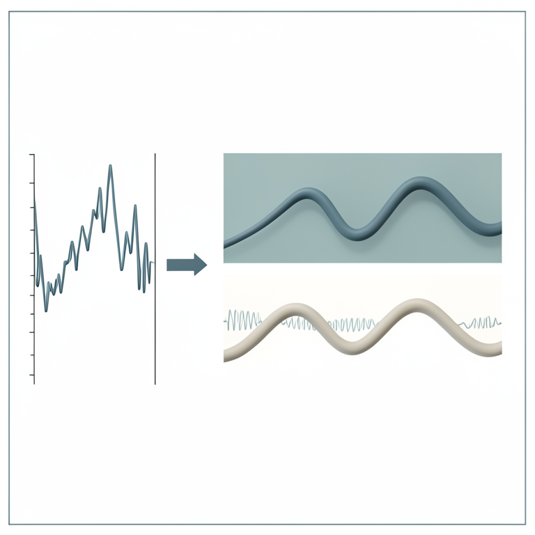
INLA Model Components
AI-generated conceptual illustration (Global satellite vegetation index time series). It explains the idea and does not show study data.
View source evidence ↗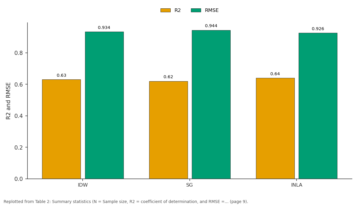
R2 and RMSE: IDW vs SG vs INLA
Replotted from Table 2 (page 9) of the original paper. Every bar is the paper's own table value.
View source evidence ↗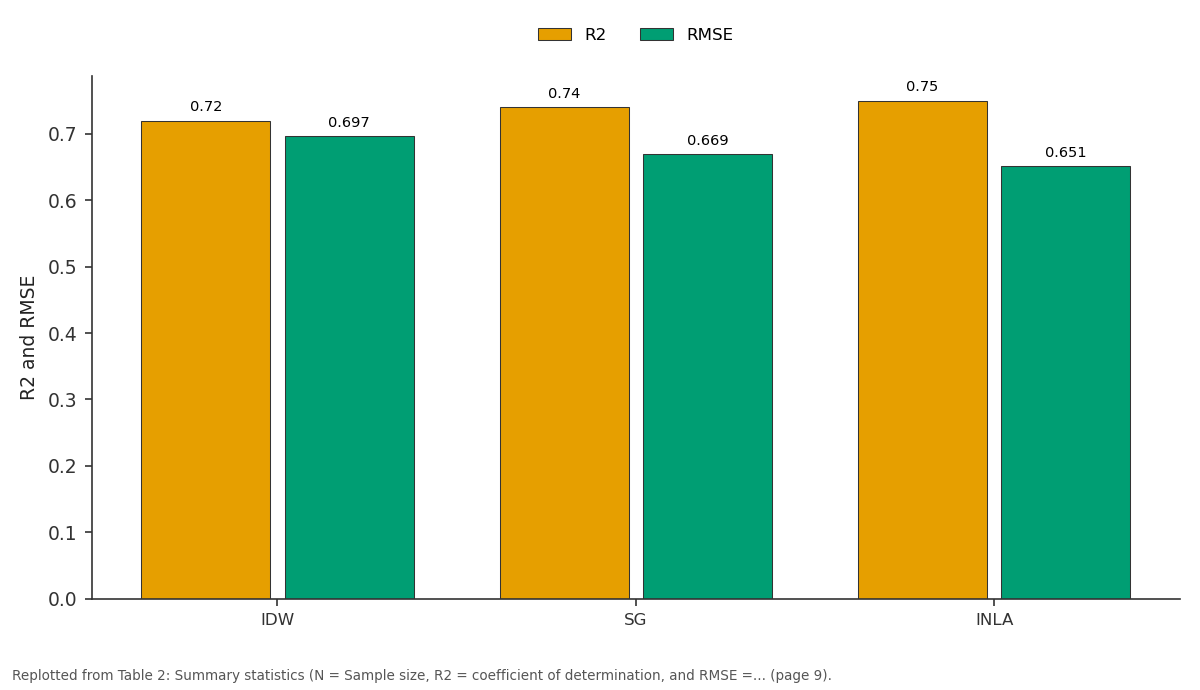
R2 and RMSE: IDW vs SG vs INLA
Replotted from Table 2 (page 9) of the original paper. Every bar is the paper's own table value.
View source evidence ↗Figures & tables
From the original paper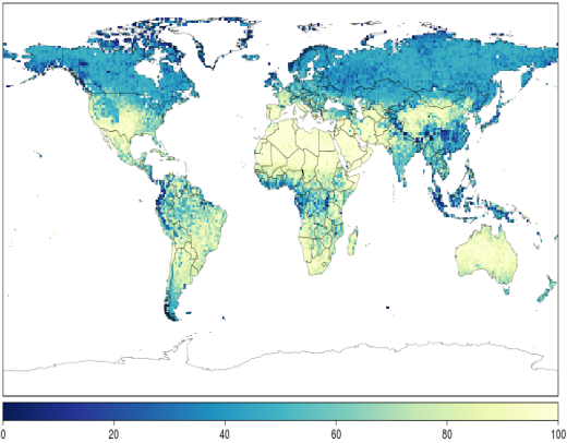 Figure 1
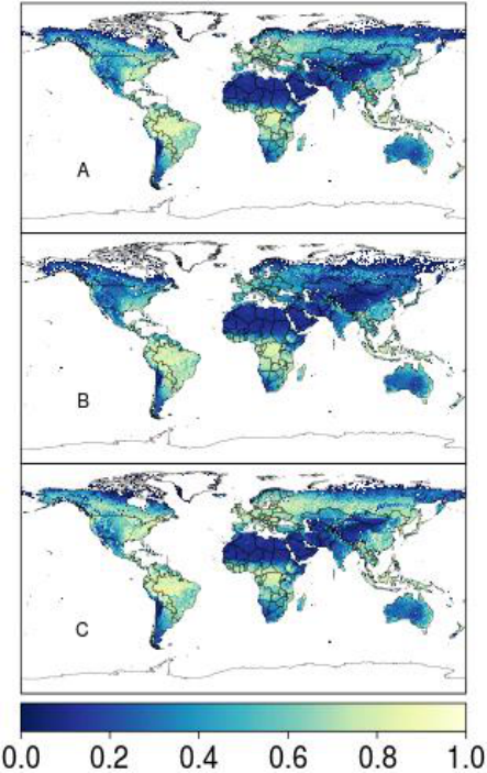 Figure 2
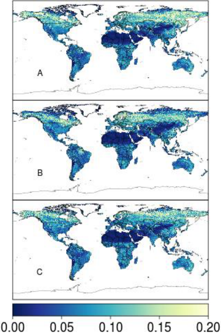 Figure 3
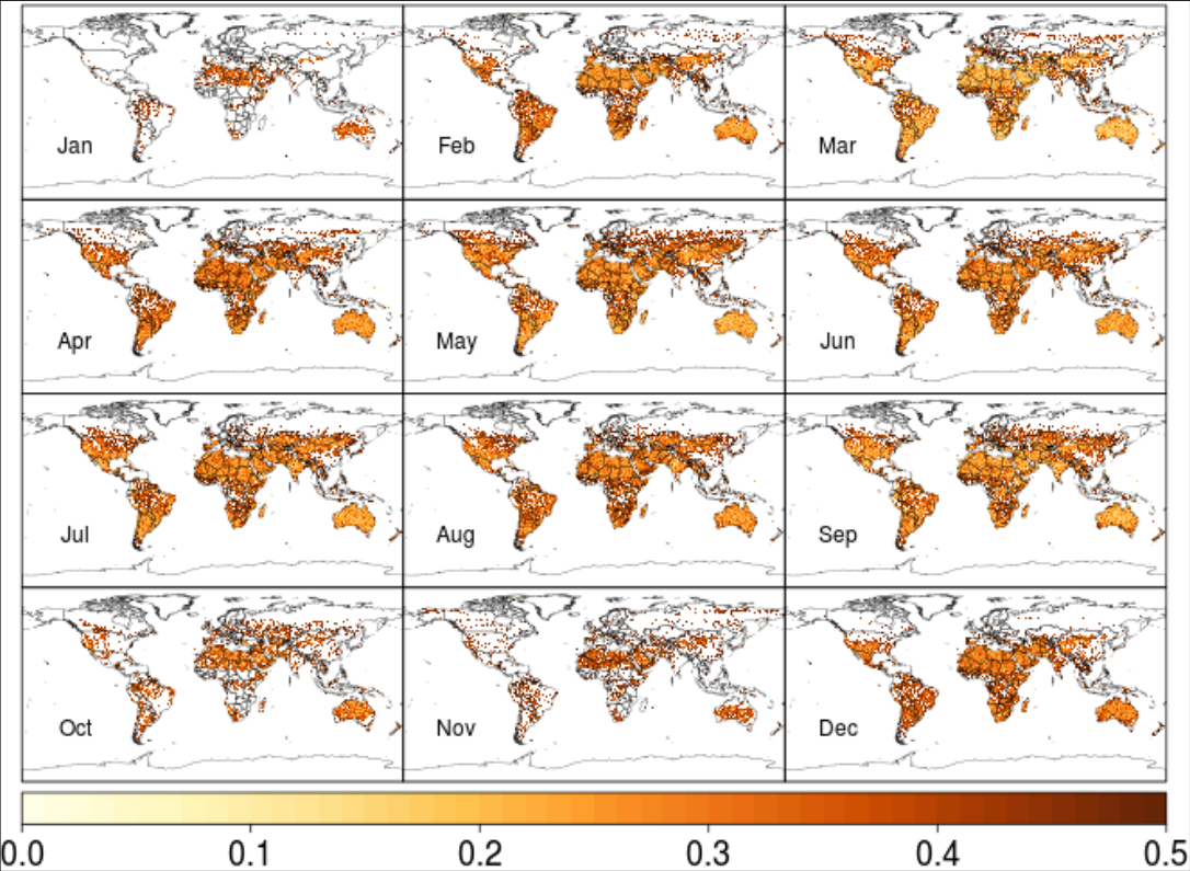 Figure 4
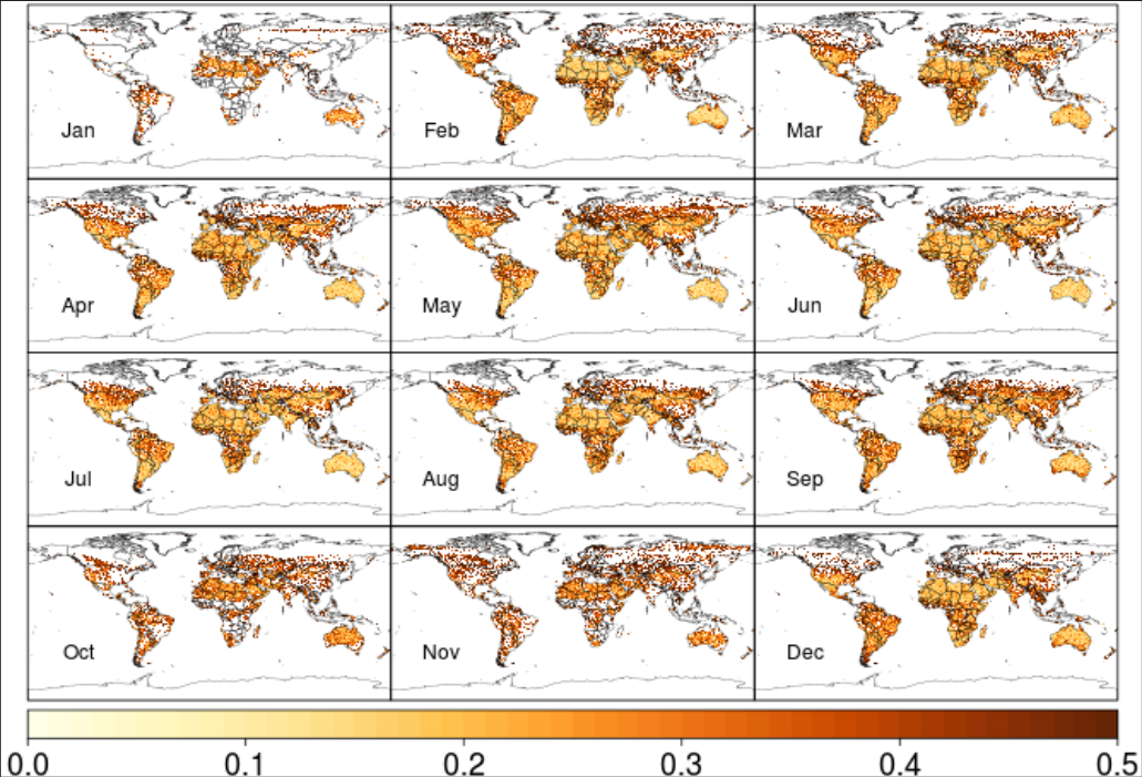 Figure 5
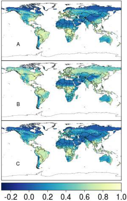 Figure 6
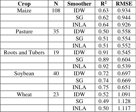 Table 2
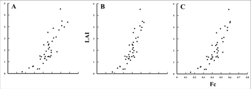 Figure 7
Introduction
The long-term monitoring of global processes and feedbacks is important for assessing the impact of climate variability and change on ecosystems (Batista et al, 1997; Weiss et al, 2004) [39] . Global vegetation records over the past three decades have facilitated studies dealing with global carbon flux, land use/cover change, and crop production estimation (Olsson et al, 2005; Xia et al, 2008) [26,40] . These vegetation records generally consist of the Normalized Difference Vegetation Index (NDVI) derived from top of canopy (TOC) visible red and nearinfrared (NIR) reflectance. In general, reflectance is detected by the Advanced Very High Resolution Radiometer (AVHRR) pre 2000, which is carried onboard the National Oceanic and Atmospheric Administration (NOAA) polar orbiting operational environmental satellites and moderate imaging spectroradiometer (MODIS) post 2000, aboard NASA's Aqua satellite (Barreto-Munoz, 2013) [2] . AVHRR is available for 30+ years, much suited for long-term climate change research studies that require going back to the 80's and 90's for more accurate global change detection (Brown et al., 2006; Marshall et al., 2016) [4,23] . However, for new studies (2000+), moderate imaging spectroradiometer (MODIS) (Fang et al., 2014; Lu et al., 2015) [7,22] is more recommended given its higher spatial, spectral resolution, and ability to eliminate background and atmosphere noises. NDVI is developed from a ratio of NIR minus visible red to NIR plus visible red to NIR plus visible red. Vegetation cover scatters (absorbs) strongly in the NIR (red) producing high NDVI compared to bare soil, which scatters strongly in both the NIR and red (Peñuelas and Filella, 1998) [28] . Aerosols, dust, Rayleigh scattering and partial cloud cover tend to increase reflectance in the NIR and lower NDVI, thus requiring additional compositing before interpretation (Holben, 1986) [14] . Major cloud contamination, particularly in the tropics, can create numerous gaps in the daily AVHRR records, eliminating approximately two-thirds of the data (Justice et al., 1991) [18] . One way to minimize the sensor and atmospheric effects is by using 15-day maximum value composites (MVC), however, gaps and inconsistencies persist, often necessitating further gap-filling and smoothing. Several long-term vegetation records exist, each with different approaches to standardize NDVI across the NOAA satellites and to account for atmospheric contamination and other effects. The Global Inventory Monitoring and Mapping Studies (GIMMS) is the most widely used NDVI product and provides long-term global data at 8 km spatial resolution (Fensholt et al, 2006) [8] . GIMMS adopts an Empirical Bayesian technique to statistically correct parts of the vegetation record that could be affected by Satellite drift and atmospheric contamination (Pinzon and Tucker, 2014; Tucker et al., 2005) [29,36] . NDVI tends to saturate more in dense vegetation and is more sensitive to soil background than enhanced vegetation index (EVI), hindering proper estimation of important biophysical parameters such as vegetation fraction and leaf area index (LAI) (Huete et al, 2002; Zhao et al, 2012) [17,24] , so a new long-term EVI product has been developed by the Vegetation Index & Phenology (VIP) Lab (Didan, 2014) [6] using AVHRR and MODIS data to overcome the limitations of NDVI. Unlike NDVI, EVI does not saturate severely in dense vegetation and incorporates a correction term to reduce the effects of soil background. The standard EVI is computed with visible red, NIR, and blue reflectance from MODIS. Since blue reflectance is not available from AVHRR, VIP developed a visible red-NIR version of EVI called EVI2 (Jiang et al., 2008) [17] . Unlike GIMMS, the VIP product which is essentially a fusion of AVHRR and MODIS undergoes partial atmospheric correction at a daily time step, before it is compositing. VIP-EVI2 and MODIS-EVI are highly correlated and perform better than their NDVI counterpart when predicting ground-based LAI (Rocha and Shaver, 2009) [31] . Due to the processing steps, however, VIP is less consistent temporally than GIMMS resulting to poor performance in trend analysis (Tian et al., 2015) [35] , and has a higher bias with ground data as noted in Marshall et al. (2016) [20] . This is due in part to the way VIP-EVI2 was reconstructed using inverse distance weighting (IDW) and linear interpolation that tended to suffer from lack of representation of variability associated with the averaged values over various regions (Zhang et al., 2014) [40] . Given that the effectiveness of compositing is limited, it has been suggested that representing bad-quality records as expressed by quality information with gaps followed by a reconstruction could improve the continuity and quality of the vegetation index data (Kandasamy et al., 2013; Pinzon & Tucker, 2014; Zhou et al., 2015) [19,29,42] . Adaptive Savitzky-Golay (SG), Whittaker-Henderson (WH) and IDW are some of the most commonly used reconstruction techniques in remote sensing. Conceptually, SG is a piece-wise regression procedure while WH is based on the minimization of a cost function describing the balance between fidelity and roughness. While SG and WH are curve-fitting techniques, IDW is a deterministic spatial interpolation technique in which values assigned to unknown points are calculated with an average, weighted by the inverse of the distance to each neighboring known point (Daly et al., 2002) [5] . As noted by Kandasamy et al. (2013) [19] , accuracy of SG and WH are significantly affected by the percentage of missing observations before reconstruction. Specifically, SG requires an a priori smoothing parameter and window size, which are assumed to be fixed while for WH, a user specified smoothing parameter is necessary to control the balance between fidelity and roughness. Vegetation index records are dynamic and as such it would be expected that multiple parameters and/or hyper-parameters would be required to characterize its variability. Consequently, a model that is driven by one (e.g. WH) or two (e.g. SG) parameters may not account for the full changes in location, variability, and shape that do occur in physical space and time (Weiss et al., 2014) [38] . An adaptive SG routine that allows the smoothing parameters to vary according to optimization criteria has been suggested by Chen et al. (2004) [7] . Further improvements have been suggested to overcome the challenge of over-smoothing or persistent roughness, but tend to perform better with pixel-level quality information characterized with large persistent good quality data. Full Bayesian inference is very flexible and does not require subjective user input and is particularly recommended for persistent large gaps with potential outliers in a long-term time series vegetation index record (Katzfuss and Cressie, 2011) [21] . Unfortunately, full Bayesian inference is computationally more intensive than other techniques and has therefore not been widely used (Pinzon and Tucker, 2014) [29] . Maximum likelihood techniques have been successfully adopted to identify optimal parameters to reduce computational constraints (e.g. empirical Bayes) improving feasibility (Pinzon and Tucker, 2014) [29] . This study considers an approximate Bayesian inferential procedure designed for latent Gaussian models to reconstruct long-term Earth observation records that is flexible and efficient (Rue et al., 2009) [32] . The Markov chain Monte-Carlo (MCMC) model convergence limitation, which accounts for most of computational demand, was overcome using an Integrated Nested Laplace Approximations (INLA) algorithm that utilizes sparse precision matrices. Physical time series components (trend, seasonal, and cyclical) are adjusted in an additive way using latent time series functions and pixel-level predictive distributions extracted as the unbiased estimate of the missing values. The paper is organized as follows: In section 2.1, EVI2 is described; in sections 2.2 and 2.3, a brief theoretical background of the Bayesian time series model using INLA is presented, and the adaptive SG routine for gap-filling and smoothing Earth observation data for comparison is briefly presented in section 2.4. An overview of the analytical methods used to compare the techniques is provided in sections 2.5 and 2.6. Results of the inter-comparison are provided in section 3.1 and 3.2, followed by a discussion of the results and conclusion in sections 4 and 5, respectively.
Data, Processing and Methods
Data, Processing and Methods
Vegetation Index & Phenology (VIP) Lab Version 3 Enhanced Vegetation Index 2 (EVI2)
We used the VIP-EVI2 record for comparison, given its potential advantage over NDVI for biophysical modeling and persistent data gaps that remain in the record after pre-processing. The data can be downloaded at http://vip.arizona.edu/viplab_data_explorer.php. VIP-EVI2 is a multi-sensor product that is partially atmospherically corrected and is available globally at a 7-day, 15-day and monthly time steps from 1981 to present at 0.05° (~5.6 km at the equator) spatial resolution (Jiang et al., 2008) [17] . For purposes of this study, 15-day VIP-EVI2 version 3 data from 1982-2011 was used. At the time of reconstruction, data analysis and writing the manuscript, a newer version of VIP-EVI2 became available, but since the purpose of this manuscript was to demonstrate the improved accuracy and lower computational demands of a Bayesian smoothing and gap-filling technique, and not the dataset itself, we retained version 3.0. Like MODIS, VIP-EVI2 includes pixel reliability (PR) bands that characterize the surface reflectance state, condition of the atmosphere and other useful information about each pixel (Didan, 2014) [6] . PR is indexed from 0 to 7 denoting best to worst data quality respectively. In its native form, Inverse Distance Weighting and Linear Interpolation (IDW) are used to reconstruct the record in order to reflect a continuous phenology curve (Didan, 2014) [6] . However, in this study, pixel level artificial gaps were created for data with corresponding PR>1, because such pixels were significantly affected by clouds, aerosols, dust, Rayleigh scattering, and other noise. This resulted in large, persistent and irregularly spaced data gaps beyond the ability of the smoothing and gap-filling methods evaluated in this study. So, these gaps were partially filled before the assessment using the MODIS filtering algorithm proposed in Xiao et al. (2003) [40] ; Marshall et al. (2016) [20] and adopted by Opiyo et al. (2013) for the tropics. The resulting pixel level percentage records available after filtering, but before applying gap-filling and smoothing techniques is provided in Figure 1. For the purpose of this study, the native gap-free record will be referred to as IDW-EVI2 while the record with missing bad-quality data referred to as VIP-EVI2. Further details on the dataset can be found in Rocha and Shaver (2009) [31] . EVI2 is derived from the following equation (1)
Reconstruction with Bayesian time series model using INLA
Vegetation index records can be classified as a hierarchical Gaussian process with linear predictor ,
Where represents the linear effects of covariates (e.g. temperature, precipitation etc.), are non-linear functions of the covariates (e.g. trend, seasonal, and cyclic effects) used to relax the linearity of the process, and are unstructured terms. This type of model is considered as a special case of the more general class of latent Gaussian models for which approximate Bayesian inference can be performed using Integrated Nested Laplace Approximations (INLA). Latent Gaussian models are considered as a sub class of structured additive regression models, in which the predictor can be expressed as a function of linear and nonlinear effects of the covariates. The vegetation index record in a given pixel is assumed to belong to an exponential family where the mean is linked to a structured additive predictor through a link function g . In this study, trend, seasonal, and cyclic terms are added to relax the linearity of the long-term time series vegetation index record. For instance, physical long-term trend effect is developed from a sequence between one and the record length. In addition, seasonal annual (short-term) variability is created and adjusted for by replicating between 1 and 12 each twice (15a and 15b) repeating the resulting sequence number of study years times. Also, long-term cyclic component adjusting for potential climate variability and change effect is developed from a replication between one and number of study years each repeated number of annual records times. The model formula is then expressed as follows;
Where is the model intercept, , , are the trend, season, and cyclic covariates respectively, n.season and n.cyclic are to be determined based on the short term and long term seasonal patterns of the process which for this study were specified as 12 and 30 respectively while the model season is as provided by default with INLA.
An autoregressive model of order 1 ( ) for the Gaussian process is defined as and autocorrelation between neighboring outcomes say , , and is expressed such that Where for . The model for seasonal variation for periodicity say for the random vector , is obtained assuming that the sums are an independent Gaussian process with precision and the density for is derived from the increments as;
Where and is the structure matrix reflecting the neighborhood structure of the model. The terms are collected in a latent field and assigned Gaussian priors such that the resulting model can be viewed as a latent Gaussian model. The posterior marginal of each element of the latent field can be expressed by;
Where, the vector denotes the hyper parameters of the model including those defining prior distributions. Applying the INLA methodology, the marginals are estimated by combining an analytical approximation with numerical integration (Rue et al., 2009) [32] . The posterior distribution for bad-quality data can be obtained by integrating out Equation 7The mean of the posterior distribution is extracted and used as the unbiased estimator to the missing/bad-quality data. The Bayesian time series procedure will be referred to as INLA method while reconstructed record using the technique referred to as INLA-EVI2.
Adaptive Savitzky-Golay Filtering technique
Performance evaluation of the Bayesian time series model was compared to the adaptive Savitzky-Golay (SG) routine proposed by The adaptive SG has been widely used to fill MODIS data. The function was implemented using the MODIS package in R. As in other reconstructions, padding was added at the beginning and end of the time series, so that smoothing and gap-filling could be performed on the tails. For the remainder of this paper, the reconstructed record using the SG procedure will be referred to as SG-EVI2.
Gap-filling and smoothing technique (global inter-comparison)
INLA-EVI2 was compared to the SG-EVI2 and IDW-EVI2 both globally and locally. The global inter-comparison was made by assessing whether IDW-EVI2 (reference record), INLA-EVI2 and SG-EVI2 were from an identical statistical distribution. The magnitude of departure from equality was measured using the distance statistic (D) two sample Kolmogorov-Smirnov (K-S) test. In addition, the ability of the SG-EVI2, INLA-EVI2, and IDW-EVI2 to produce consistent records was evaluated using long-term trend analysis based on a non-parametric Thiel-Sen (T-S) regression (Fensholt and Proud, 2012) [9] masked for significance at alpha=0.05 estimated using a seasonally corrected Mann-Kendall trend test.
Goodness-of-fit test with two-sample Kolmogorov-Smirnov test
The two-sample Kolmogorov-Smirnov (K-S) test was employed to assess degree of similarity between IDW-EVI2 (reference record), SG-EVI2 and INLA-EVI2 time series records. It is based on a statistical distance statistic (D) procedure involving two sample records, with a low value of D statistic (p-value > 0.05), suggesting increased accuracy of the method. High value of D (D > 0.5) tended to produce low p-values (p-value < 0.05) suggesting varied statistical distribution. The non-parametric technique is a widely used statistical procedure that compares two empirical continuous distribution functions. The D statistic is computed from the maximum distance between the two empirical distributions based on the ranks. Although the test analyzes the actual data, it is equivalent to analysis of ranks which tend to be robust and desirable when the underlying statistical distribution of the records is not well understood.
Long-term Trend Analysis with Theil-Sen Regression
The ability of the smoothing techniques to produce consistent long-term time series records was evaluated using the Theil-Sen (T-S) regression approach. It computes pairwise slopes of all datapoints and computes the median slope of those values. The median slope value becomes unbiased slope estimate.
Mann-Kendall Slope Significance Testing
Statistical significance of the T-S regression slope estimates was evaluated using the Mann-Kendall (M-K) test. Slope significance with M-K test was considered due to its flexibility when the record is suspected to be non-linear with potential outliers. It is a nonparametric distribution free test for monotonic trends and correlation analysis. The test statistic is then provided by the number of positive differences minus the number of negative differences (Verbesselt et al., 2010) [35] . A positive test statistic implies that observations obtained later in time tend to be larger than observations made earlier, while a negative test statistic implies that the observations made later tend to be smaller than those made earlier (Tian et al., 2015) [35] . For every test statistic, a probability value was extracted and used to mask T-S slope estimates for significance at alpha=0.05.
Gap-filling and smoothing technique (local inter-comparison)
The new smoother was compared to the optimization routine locally (subset of pixels) using a newly developed database of 1,459 in situ LAI measurements for major field crops (alfalfa, barley, canola, cotton, garlic, maize, onion, pasture, potato, rice, soybean, sugar beet, and wheat) on five continents (Asia, Australia, Europe, North America, and South America). The database was compiled from several sources of LAI measurements made using destructive and non-destructive (optical) methods spanning the evaluation period. NDVI and other vegetation indices are widely used to compute LAI in global change studies (Fensholt et [10,12,30,22] , so Landsat reflectance data (30 m resolution) was later processed to compute NDVI and other vegetation indices, and paired with the in situ LAI data to evaluate the universality of the vegetation index-LAI relationship. Further details on this dataset can be found in Kang et al. (2016) [20,23] . Since the relationship between in situ and coarse resolution vegetation indices and LAI is typically non-linear (Asrar et al., 1992; Myneni et al., 2002; Friedl et al., 1995; Gutman and Ignatov, 1998; Sellers, 1985) [1,25,11,13] , Landsat EVI2 pixels within each IDW-EVI2 pixel were used to downscale IDW-EVI2, SG-EVI2, and INLA-EVI2 data using the vegetation fraction (F C ) procedure suggested by Hwang et al. (2011) [15] . Unlike the vegetation index-LAI relationship, the vegetation index -F C relationship is quasi-linear; meaning F C estimated with a coarse resolution pixel is approximately equal to the average of F C estimating from corresponding higher resolution pixels. In Hwang et al. (2011) [15] , this relationship was used to downscale MODIS (250 m) NDVI with Landsat NDVI. The technique is ratio-based and parameterized for flat and complex terrain. Since the LAI measurements were retrieved from large and flat agroecosystems, we used the simple proportionality formula for each data pair to convert IDW-EVI2 to downscaled (30 m) F C for comparison with in situ LAI:
Where α is the proportionality constant, F C, Landsat is the vegetation fraction computed from Landsat EVI2, and EVI2 Landsat is EVI2 derived from Landsat top of atmosphere reflectance. We computed F C for Landsat with the formula developed for the MODIS Evapotranspiration Model (MOD16)
Where EVI2 min equals 0.05 and represents EVI2 for bare soil (LAI→0) and EVI2 max equals 0.95 and represents EVI2 for dense vegetation (LAI→∞). IDW-EVI2 F C was computed by multiplying IDW-EVI2 by the proportionality constant. In some cases, more than one Landsat pixel fell within an IDW-EVI2 pixel in space and time. In these cases, F C, Landsat values were averaged before downscaling. In order to compare SG-EVI2 and INLA-EVI2, Landsat-LAI pairs were removed and then the corresponding time series were smoothed and gap-filled. Standard linear regression statistics (coefficient of determination-R 2 and Root Mean Squared Error-RMSE) were computed from the raw IDW-EVI2 data, SG-EVI2, and INLA-EVI2 versus LAI. Transformations were deemed unnecessary, because the data exhibited near linear relationships (not shown).
Results
Results
Global inter-comparison
Pixel level means and standard deviations were obtained tocompare the distribution of SG-EVI2 and INLA-EVI2 to IDW-EVI2 (Figure 2). SG-EVI2 tended to over-predict IDW-EVI2, while INLA-EVI2 tended to under-predict IDW-EVI2 as shown in Figure 2. Although the absolute magnitudes were different, INLA-EVI2 showed a higher level of agreement with IDW-EVI2 in terms of the overall distribution of estimated values than SG-EVI2. The greatest difference between the SG-EVI2 and INLA-EVI2 was at the extreme Northern latitude in which the mean predicted values appear lowest and most variable (Figure 3). The two sample K-S test was used to assess whether INLA-EVI2 and SG-EVI2 had identical distributions to IDW-EVI2 (in terms of medians, variability, and shape). The null hypothesis is that the IDW-EVI2 and SG-EVI2 or INLA-EVI2 was sampled from populations with identical distributions. The magnitude of the D statistic expresses indirectly, the degree of violation of the null hypothesis with higher values (p < 0.05) suggesting that the two reconstructed records are from different statistical distributions.
Overall goodness-of-fit on a monthly basis for SG-EVI2 and INLA-EVI2 are shown in Figure 4 and Figure 5, respectively. In each case, pixel level K-S estimates with p-value < 0.05 were masked for display purposes. As shown in Figures 4 and5, the patterns in correlations between IDW-EVI2 (reference), SG-EVI2, and INLA-EVI2 based on the D statistic were fairly identical. Nevertheless, INLA-EVI2 and IDW-EVI2 appears to be more similar as suggested by lowest D statistic. The highest level of correlation was found at mid-latitudes throughout much of the year, while average correlations were found during green-up and summer months at northernmost latitudes (March-April-May and June-July-August) and the poorest correlations were observed during brown-down (fall) months at northernmost latitudes (October-January). Overall, INLA provided better model fit with over 70% of pixels reporting D <0.2 while the SG method produced D between 0.1 and 0.4 and a majority (D > 0.5) masked to express varied distribution. D > 0.5 (varied distribution) was most prevalent during boreal and austral summer months (October-February) for both the SG-EVI2 and the INLA-EVI2 approach even though the degree of variability appears highest with the SG-EVI2.
The T-S regression model masked for significance using the M-K test was used to study the annual trends in VIP-EVI2 with each technique (Figure 6). Positive values indicate a greening trend, while negative values indicate a browning trend. Overall, greening trends were more prevalent at mid-latitude and least significant at extreme high latitudes. INLA-EVI2 and IDW-EVI2 were closer in terms of trend magnitude and direction than SG-EVI2 and IDW-EVI2. The greatest difference in the techniques appear to be in their degree of sensitivity to weak browning/greening trends in which SG appear to be least sensitive as expressed by large number of insignificant trends at extreme high latitudes.
Local inter-comparison
Of the original 1,459 Landsat-LAI pairs, only 319 samples remained for comparison due to overlap between AVHRR and Landsat pixels in space and time. Initially, LAI and downscaled IDW-EVI2 statistics were computed for the pooled (all crops) data, but this led to poor and insignificant relationships, so statistics were computed instead on a per-crop basis. On a per-crop basis, sample sizes were small, so additional data points for some crops were omitted from the analysis, including: barely, canola, cotton, and rice. In order to increase the sample sizes of the remaining crop, two aggregations were made: alfalfa was included with pasture and garlic, onion, potato, and sugar beet were combined to form a "roots and tubers" category. After these processing steps, 225 samples remained for analysis. Based on the summary statistics used for the global comparison, INLA-EVI2 again showed the strongest correlation with LAI compared to SG-EVI2 and IDW-EVI2 (Table 1). For maize, pasture, roots and tubers, soybean, and wheat, INLA explained an additional 2%, <1%, 3%, 1%, and 1% of LAI variance than SG-EVI2, respectively. IDW showed minor improvements over SG-EVI2 for Maize (ΔR 2 =0.01) and Roots and Tubers (ΔR 2 =0.02), and under-performed INLA with the exception of wheat (ΔR 2 =0.02). As illustrated in Figure 7 for soybean, INLA consistently reproduced strong linear relationships over a similar range as IDW-EVI2 compared to SG-EVI2. SG-EVI2 had a lower dynamic range, which lead to a steeper slope and small, but lower correlations with in situ LAI. [19] , the upper envelop approach in the SG-EVI2 tends to overestimate vegetation index values in regions that are least affected by atmospheric cloud cover, because it preserves the upper envelope (VIP-EVI2 maxima) of the time series. Since the optimization routine produced a lower dynamic range than INLA-EVI2, minima were higher as well. In the global comparison, over 70% of the INLA-EVI2 and IDW-EVI2 goodness-of-fit test resulted in D < 0.5. While the distribution of D statistic for SG-EVI2 and IDW-EVI2 was comparable, it tended to result in higher D's suggesting different statistical distributions. The level of disagreement based on the D statistic (D > 0.5) was highest at northern extremes during winter and least during summer months at midlatitudes. The distribution of significant D statistic (disagreements not attributable to chance) was considerably higher in SG-EVI2/IDW-EVI2 than INLA-EVI2/IDW-EVI2. Coincidentally, the level of agreement between predicted values and corresponding IDW-EVI2 appear to decrease as the percentage gaps in VIP-EVI2 increases. The finding is consistent with Rusticus and Lovato (2014) [33] who noted that the overall power of equivalence testing is strongly influenced by sample size. The Lowest agreement was noted during winter months when the percentage of good quality data was lowest and highest during summer months when good quality data was most abundant. The impact of percentage gaps on reconstruction was more severe and heterogeneous for SG-EVI2 than INLA-EVI2, which is confirmed by Kandasamy et al. (2013) [19] , who observed that among the techniques they compared, SG was more sensitive to the number and length of data gaps. Seasonality was less apparent in the southern hemisphere, which was likely due to the greater proportion of water (i.e. less continentally).
A non-parametric regression model based on the T-S slope masked for significance with a seasonal Mann-Kendall trend test was used to determine annual trends for each smoothing technique. The technique was employed to circumvent the independence assumption and potential effects of outliers, which in the presence of serial autocorrelation, tends to pose a challenge to matrix algebra. Despite some regional differences in areas at high latitudes with many data gaps, there was a high level of agreement between annual trends produced from the smoothing techniques compared to IDW-EVI2 in this study and those produced from GIMMS and MODIS NDVI records in Fensholt et al. (2012) [9] and in Marshall et al. (2016) [20] . Each technique produced positive (green-up) trends over much of the globe. Generally, the greening has been attributed in previous studies to an increase in and extension of primary plant production (when light and moisture are not limiting factors) in response to global warming. Despite T-S slope estimates associated with the optimization routine being consistently higher (depicting a high rate of greening), INLA-EVI2 showed more brown-down/green-up trends at extreme latitudes, while SG-EVI2 showed more negative (browning) trends which are slightly higher in absolute terms. Marshall et al. (2016) [20] confirms the INLA-EVI2 results, revealing that trends can be heterogeneous in both space and time, due to droughts, fires, pests, land cover change, and climate-land feedbacks. In addition, discontinuities in the data record, transitions in annual trends, and differences in the trend analysis approach used, can make comparisons particularly difficult at these latitudes.
Unique to this study, the smoothing techniques developed from coarse resolution Earth observation data were compared using ground-based data. [15] and the in situ database created by Kang et al. (2016) [20,23] can be used in conjunction with other in situ databases, such as the woody plant database (Iio et al., 2014) [16] in the future, to evaluate the updated VIP version 4 and other records (e.g. MODIS) with various gap-filling and smoothing approaches. The primary disadvantage of full Bayesian techniques especially using MCMC and a reason they have not been widely used for smoothing in the remote sensing community, is that they are computationally more intensive. The findings reveal desirable benefits that come with full Bayesian smoothing (e.g. being less severely impacted by the large fraction and length of missing data) compared to the commonly used curve-fitting techniques. INLA approach is limited to latent Gaussian models (Rue et al., 2009) [32] , unlike MCMC methods which are very general, flexible and can effectively be applied to nearly any model. However, in some cases, it is difficult to assess MCMC convergence to the target posterior distribution, resulting to inference from a false positive posterior distribution. It is our view that the main benefit of the new gap-filling and smoothing procedure is computational, a short cut to full Bayesian inference with simulation based routines which is near impossible for complex models despite having desirable properties.
Conclusion
The research presented in this study highlights the important role a full Bayesian time series model with INLA can play in reconstructing Long-term Earth observation based vegetation index records where the underlying processes are not well understood and contain several outliers and discontinuities. Specifically, this study showed, using AVHRR-MODIS fused records and in situ data that a full Bayesian time series smoothing procedure is less severely impacted by missing data than the commonly used SG procedure. Performance assessment with K-S test suggests more comparable findings between SG-EVI2 and INLA-EVI2 during summer but more different estimates during winter. This is reflected by the high proportion of pixels with high distance statistic (D > 0.5) which indicates high level of disagreement with IDW-EVI2 (reference record). In particular, such pixels were more erratic during winter for SG-EVI2 but were fewer and fairly distributed across the months of the year for INLA-EVI2. The good performance of INLA-EVI2 was also demonstrated by its ability to detect long-term annual trends. While annual trend analysis with INLA-EVI2 and IDW-EVI2 were comparable across the globe, trends with SG-EVI2 were different in regions negatively impacted by atmospheric contaminations. Such Poor and largely non-significant long-term annual trends for SG-EVI2 were noted in extreme high latitude (e.g. Canada, Russia), Brazil, parts of Australia and other regions that are either water or largely Forest ecosystem (e.g. Congo). The good performance of INLA-EVI2 was further validated by its ability to correctly estimate ground observed LAI data taken for major crop areas. Of the five major crop areas (maize, pasture, roots and tubers, soybean, and wheat) considered, INLA-EVI2 predicted the in situ LAI data more precisely than the alternative records (SG-EVI2 and IDW-EVI2) for Maize, pasture, roots and tubers, and soybean, producing highest R 2 and lowest RMSE. Therefore, we suggest considering Bayesian time series model under INLA to gap-fill and smooth long-term Earth observation based vegetation index. The procedure is highly flexible for a large class of statistical models (http://www.r-inla.org/). Alternative latent models available under INLA can also be tested for the time series components to assess performance difference in terms of improved accuracy. However, if computational resources are heavily restricted, we recommend IDW and linear interpolation due to its fairly good performance. However, SG procedure could be adopted in regions less impacted by atmospheric contamination given its relatively high accuracy, simplicity and computational efficiency.
Acknowledgements
Acknowledgements
Figures and tables from the paper
| Crop | N | Smoother | R2 | RMSE |
|---|---|---|---|---|
| Maize | 108 | IDW | 0.63 | 0.934 |
| SG | 0.62 | 0.944 | ||
| INLA | 0.64 | 0.926 | ||
| Pasture | 35 | IDW | 0.50 | 0.558 |
| SG | 0.51 | 0.554 | ||
| INLA | 0.51 | 0.552 | ||
| Roots and Tubers | 19 | IDW | 0.91 | 0.545 |
| SG | 0.89 | 0.604 | ||
| INLA | 0.92 | 0.539 | ||
| Soybean | 40 | IDW | 0.72 | 0.697 |
| SG | 0.74 | 0.669 | ||
| INLA | 0.75 | 0.651 | ||
| Wheat | 23 | IDW | 0.52 | 1.091 |
| SG | 0.49 | 1.128 | ||
| INLA | 0.50 | 1.117 |
Table text extracted from the original PDF; superscript letters are shown inline. The original table image is below.
View original table image
References
41 in the original paper- Asrar G, Myneni RB, Choudhury BJ. Spatial heterogeneity in vegetation canopies and remote sensing of absorbed photosynthetically active radiation: A modeling study. Remote Sens. Environ. 1992; 41:85-103. doi:10.1016/00344257(92)90070-Z
- Barreto-Munoz A. Multi-Sensor Vegetation Index and Land Surface Phenology Earth Science Data Records in Support of Global Change Studies: Data Quality Challenges and Data Explorer System, 2013.
- Batista GT, Shimabukuro YE, Lawrence WT. The long-term monitoring of vegetation cover in the Amazonian region of northern Brazil using NOAA-AVHRR data. Int. J. Remote Sens. 1997; 18:3195-3210. doi:10.1080/0 14311697217044
- Brown ME, Pinzón JE, Didan K, Morisette JT, Tucker CJ. Evaluation of the Consistency of Long-Term NDVI Time Series Derived From AVHRR, and Landsat ETM + Sensors. 2006; 44:1787-1793.
- Daly C, Gibson WP, Taylor GH, Johnson GL, Pasteris P. A knowledge-based approach to the statistical mapping of climate. Clim. Res. 2002; 22:99-113. doi:10.3354/cr022099
- Didan K. Multi-satellite Earth science data record for studying global vegetation trends and changes. Int. Geosci. Remote Sens. Symp, 2014.
- Fang X, Zhu Q, Chen H, Ma Z, Wang W, Song X, et al. Analysis of vegetation dynamics and climatic variability impacts on greenness across Canada using remotely sensed data from 2000 to 2009. J. Appl. Remote Sens. 2014; 8:836-66. doi:10.1117/1.jrs.8.083666
- Fensholt R, Nielsen TT, Stisen S. Evaluation of AVHRR PAL and GIMMS 10-day composite NDVI time series products using SPOT-4 vegetation data for the African continent. Int. J. Remote Sens. 2006; 27:2719-2733. doi:10.1080/01431160600567761
- Fensholt R, Proud SR. Evaluation of Earth Observation based global long term vegetation trends -Comparing GIMMS and MODIS global NDVI time series. Remote Sens. Environ. 2012; 119:131-147. doi:10.1016/j.rse.2011.12.015
- Fensholt R, Sandholt I, Rasmussen MS. Evaluation of MODIS LAI, fAPAR and the relation between fAPAR and NDVI in a semi-arid environment using in situ measurements. Remote Sens. Environ. 2004; 91:490-507.
- Friedl MA, Davis FW, Michaelsen J, Moritz MA. Scaling and uncertainty in the relationship between the NDVI and land surface biophysical variables: An analysis using a scene simulation model and data from FIFE. Remote Sens. Environ. 1995; 54:233-246. doi:10.1016/0034-4257(95)00156-5
- Gitelson AA, Peng Y, Huemmrich KF. Relationship between fraction of radiation absorbed by photosynthesizing maize and soybean canopies and NDVI from remotely sensed data taken at close range and from MODIS 250m resolution data. Remote Sens. Environ. 2014; 147:108-120. doi:10.1016/j.rse.2014. 02.014
- Gutman G, Ignatov A. The derivation of the green vegetation fraction from NOAA/AVHRR data for use in numerical weather prediction models. Int. J. Remote Sens. 1998; 19:1533-1543.. doi:10.1080/014311698215333
- Holben BN. Characteristics of maximum-value composite images from temporal AVHRR data, 1986, 37-41. doi:10.1080/01431168608948945
- Hwang T, Song C, Bolstad PV, Band LE. Downscaling real-time vegetation dynamics by fusing multi-temporal MODIS and Landsat NDVI in topographically complex terrain. Remote Sens. Environ. 2011; 115:2499-2512. doi:10.1016/j.rse.2011.05.010
- Iio A, Hikosaka K, Anten NPR, Nakagawa Y, Ito A. Global dependence of field-observed leaf area index in woody species on climate: a systematic review. Glob. Ecol. Biogeogr. 2014; 23:274-285.
- Jiang Z, Huete A, Didan K, Miura T. Development of a two-band enhanced vegetation index without a blue band. Remote Sens. Environ. 2008; 112:3833-3845. doi:10.1016/j.rse.2008.06.006
- Justice CO, Eck TF, TANRÉ D, Holben BN. The effect of water vapour on the normalized difference vegetation index derived for the Sahelian region from NOAA AVHRR data. Int. J. Remote Sens. 1991; 12:1165-1187.
- Kandasamy S, Neveux P, Verger A, Buis S, Weiss M, Baret F. Improving the Consistency and Continuity of MODIS 8 Day Leaf Area Index Products. Int. J. Electron. Telecommun. 2012; 58:141-146. doi:10.2478/v10177-012-0020-8
- Kang Y, Özdoğan M, Zipper S, Román M, Walker J, Hong S, Marshall M et al. How Universal Is the Relationship between Remotely Sensed Vegetation Indices and Crop Leaf Area Index? A Global Assessment. Remote Sens. 2016; 8:597. doi:10.3390/rs8070597
- Katzfuss M, Cressie N. Spatio-temporal smoothing and EM estimation for massive remote-sensing data sets. J. Time Ser. Anal. 2011; 32:430-446.
- Lu L, Kuenzer C, Wang C, Guo H, Li Q. Evaluation of three MODIS-derived vegetation index time series for dryland vegetation dynamics monitoring. Remote Sens. 2015; 7:7597-7614. doi:10.3390/rs70607597
- Marshall M, Okuto E, Kang Y, Opiyo E, Ahmed M. Global assessment of Vegetation Index and Phenology Lab (VIP) and Global Inventory Modeling and Mapping Studies (GIMMS) version 3 products. Biogeosciences. 2016; 13:625-639.
- Mu Q, Heinsch FA, Zhao M, Running SW. Development of a global evapotranspiration algorithm based on MODIS and global meteorology data. Remote Sens. Environ. 2007; 111:519-536. doi:10.1016/j.rse.2007 .04.015
- Myneni RB, Hoffman S, Knyazikhin Y, Privette JL, Glassy J, Tian Y et al. Global products of vegetation leaf area and fraction absorbed PAR from year one of MODIS data. Remote Sens. Environ. 2002; 83:214-231. doi:10.1016/S00344257(02)00074-3
- Olsson L, Eklundh L, Ardö J. A recent greening of the Sahel -Trends, patterns and potential causes. J. Arid Environ. 2005; 63:556-566. doi:10.1016/j.jaridenv.2005 .03.008
- Opiyo EO, Ngigi T, Nduati E, Mang M. A Prototype online system to process and visualize phenology parameters for Kenya : Case study of Bunguma county, 2013.
- Peñuelas J, Filella L. Visible and near-infrared reflectance techniques for diagnosing plant physiological status. Trends Plant Sci. 1998; 3:151-156. doi:10.1016/S1360-1385(98)01213-8
- Potithep S, Nasahara NK, Muraoka H, Nagai S, Suzuki R, Science E. What Is the Actual Relationship Between Lai and Vi in a Deciduous Broadleaf Forest ? Remote Sens. Spat. Inf. Sci. 2010; 38:609-614.
- Rocha AV, Shaver GR. Advantages of a two band EVI calculated from solar and photosynthetically active radiation fluxes. Agric. For. Meteorol. 2009; 149:1560-1563. doi:10.1016/j.agrformet.2009.03.016
- Rue H, Martino S, Chopin N. Approximate Bayesian inference for latent Gaussian models by using integrated nested Laplace approximations. J. R. Stat. Soc. Ser. B (Statistical Methodol. 2009; 71:319-392. doi:10.1111/j.1467-9868.2008.00700.x
- Rusticus SA, Lovato CY. Impact of Sample Size and Variability on the Power and Type I Error Rates of Equivalence Tests : A Simulation Study. Pract. Assesment, Res. Eval. 2014; 19.
- Sellers PJ. Canopy reflectance, photosynthesis and transpiration. Int. J. Remote Sens. 1985; 6:1335-1372. doi:10.1080/01431168508948283
- Tian F, Fensholt R, Verbesselt J, Grogan K, Horion S, Wang Y. Evaluating temporal consistency of long-term global NDVI datasets for trend analysis. Remote Sens. Environ. 2015; 2. doi:10.1016/j.rse.2015.03.031
- Tucker C, Pinzon J, Brown M, Slayback D, Pak E, Mahoney R, et al. An extended AVHRR 8-km NDVI dataset compatible with MODIS and SPOT vegetation NDVI data. Int. J. Remote Sens. 2005; 26:4485-4498. doi:10.1080/01431160500168686
- Wang Q, Adiku S, Tenhunen J, Granier A. On the relationship of NDVI with leaf area index in a deciduous forest site. Remote Sens. Environ. 2005; 94:244-255. doi:10.1016/j.rse.2004.10.006
- Weiss DJ, Atkinson PM, Bhatt S, Mappin B, Hay SI, Gething PW. ISPRS Journal of Photogrammetry and Remote Sensing An effective approach for gap-filling continental scale remotely sensed. ISPRS J. Photogramm. Remote Sens. 2014; 98:106118. doi:10.1016/j. isprsjprs. 2014.10.001
- Weiss JL, Gutzler DS, Coonrod JEA, Dahm CN. Long-term vegetation monitoring with NDVI in a diverse semi-arid setting, central New Mexico, USA. J. Arid Environ. 2004; 58:249-272. doi:10.1016/j.jaridenv.2003.07.001
- Xiao X, Braswell B, Zhang Q, Boles S, Frolking S, Moore B. Sensitivity of vegetation indices to atmospheric aerosols: Continental-scale observations in Northern Asia. Remote Sens. Environ. 2003; 84:385-392. doi:10.1016/S00344257(02)00129-3
- Yu H, Xu J, Okuto E, Luedeling E. Seasonal response of grasslands to climate change on the Tibetan Plateau. PLoS One. 2012; 7:e49230. doi:10.1371/journal.pone. 0049230
- Zhou J, Jia L, Menenti M. Remote Sensing of Environment Reconstruction of global MODIS NDVI time series : Performance of Harmonic ANalysis of Time Series (HANTS). Remote Sens. Environ, 2015. doi:10.1016/j.rse.2015.03.018