
Research article · 2018 · Full text
International Journal of Statistics and Applied MathematicsPairwise comparative analysis of two reliability models with regard to undertaking the failed unit by ordinary or expert repairman with the concept of instruction and replacement time
Volume 3(1) · Pages 511–513
Research areasReliability and Maintenance OptimizationEngineering Diagnostics and ReliabilityFatigue and fracture mechanics
Abstract
Author-writtenThe present paper deals with pairwise comparative analysis of two reliability models with regard to undertaking the failed unit by ordinary or expert repairman in the concept of instruction and replacement time. In model-1 if at the time of completion of the repair of a failed unit by the expert the second unit is found in failed state, it is also repaired by the expert. In model-2 every failed unit first goes under the repair of ordinary repairman who starts repair after getting instruction from the expert.
Summary
Source-checkedPlain-language reading of the full paper, prepared with AI and checked against the text. Each point links to the authors' own words.
Why it matters
- Redundancy, specifically through two-unit standby systems, is a widely used method to improve system reliability. View evidence ↗
- Reliability studies often distinguish between ordinary and expert repairmen, as ordinary repairmen may be unable to perform complex repairs. View evidence ↗
- Ordinary repairmen can accidentally damage units during repair attempts, potentially leading to a state where the unit must be replaced entirely. View evidence ↗
What they did
- The research investigates a two-unit cold standby system incorporating instruction and replacement policies. View evidence ↗
- The models assume exponential distributions for failure times, while other time distributions are treated as arbitrary. View evidence ↗
- System effectiveness and profit were evaluated using Semi-Markov Processes and the regenerative point technique. View evidence ↗
What they found
- The difference in profit between the two models (P62-P61) increases as the cost C2 increases and is higher when cost C8 is higher. View evidence ↗
- When C8 is 200, Model 2 is more profitable than Model 1 if the cost C2 exceeds 8608.84. View evidence ↗
- When C8 is 400, Model 2 is more profitable than Model 1 if the cost C2 exceeds 8478.91. View evidence ↗
- When C8 is 600, Model 2 is more profitable than Model 1 if the cost C2 exceeds 8340.12. View evidence ↗
- The profit difference (P62-P61) increases with higher values of probability p1 but decreases as probability b2 increases. View evidence ↗
- If probability b2 is 0.3 or less, Model 2 is consistently more profitable than Model 1 regardless of the value of p1. View evidence ↗
- When b2 is 0.5, Model 2 is more profitable than Model 1 only if p1 is greater than 0.037. View evidence ↗
- When b2 is 0.7, Model 2 is more profitable than Model 1 only if p1 is greater than 0.098. View evidence ↗
What it means
- The authors conclude that no single reliability model is superior in all scenarios; the best model depends on the specific situational parameters. View evidence ↗
- The authors suggest that this comparative analysis can serve as a guide for companies deciding which system to implement based on their current conditions. View evidence ↗
Figures & tables
From the original paper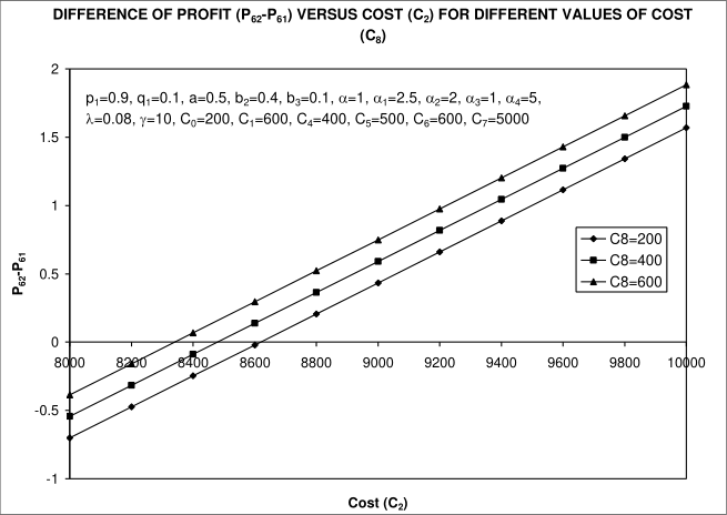 Figure 1
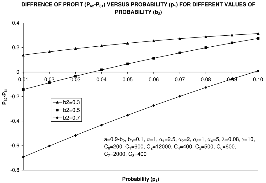 Figure 2
Introduction
In order to enhance the reliability, concept of redundancy is used in various systems. As a result, two-unit standby systems have widely been studied in the field of reliability. Concept of two types of repairman has been considered in some of these studies including [1][2][3][4][5] wherein one of the repairman had been taken as an ordinary and the other as an expert. The ordinary repairman may not be able to do some complex repairs and then an expert comes. Long stay of the expert with the system may be costly and hence idea of instruction time was introduced by Kumar et al. [3] There may also be situations when the ordinary repairman even after getting the instruction may damage the failed unit during his try for repair. This leads to the unit in more degraded stage and sometimes to a stage where we are left with no other option but to replace it by a new one. The purpose of the present study is: i) To introduce redundancy ii) To introduce a new type of repair policy which is defined as: "when the ordinary repairman makes the unit damaged and leads it to more degraded stage due to mishandling, it is undertaken by the expert at much earlier stage than the stage at which its repair has been started by the ordinary repairman" iii) To make the replacement when the failed unit is made no more repairable by the ordinary repairman iv) To reduce the stay of the expert. The present paper, therefore, investigates two-unit cold standby system introducing the aforesaid repair policy together with instruction and replacement. In model-1 if at the time of completion of the repair of a failed unit by the expert the second unit is found in failed state, it is also repaired by the expert and in model-2 the additional assumptions taken for the model is that every failed unit first goes under the repair of ordinary repairman who starts repair after getting instructions from expert. Failure times are assumed to follow exponential distributions whereas other time distributions are arbitrary. Other assumptions are as usual. Both the systems have been analysed by making use of Semi-Markov Processes and regenerative point technique in Reference 6 and Reference 7. Various measures of system effectiveness including profit incurred have been evaluated.
Various cutoff points for various rates / costs / probabilities, prior or beyond which the system is profitable, have been obtained. However, no model is best in every situation. A model may be better in some situations but worse in some other situations. So it is highly significant to make the comparative study of the models taking two at a time to know under which situation one is better than the other so far as the economical aspect concerned.
Comparative analysis of model discussed in reference 6 and reference 7 Pairwise comparative analysis of the models through graphs is carried out for the same particular cases as taken in the previous papers for concerned models. The assumed values for various rates/costs/probabilities have been mentioned along with graphs. Let P 61 be the profit of the model discussed in the Reference 6 and P 62 be the profit of the model discussed in Reference 7. Let us now compare the models (taking two at a time) through graphs on the basis of profit aspect. Two models of two-unit cold standby systems with the concept of replacement and instruction rate discussed in reference 6 and reference 7 have been compared by plotting the two graphs. (A) Behaviour of the difference between profits P 62 and P 61 with respect to cost (C 2 ) for different values of cost (C 8 ) is shown as in Fig. 1. Following observations can be made: (i) The difference increases with increase in values of cost (C 2 ) and becomes higher for higher values of C 8 . (iii) For C 8 = 400, (P 62 P 61 ) > or = or < 0 according as C 2 > or = or < 8478.91. So, Model 2 is better or worse than Model 1 if C 2 > or < 8478.91. Both the models are equally good if C 2 = 8478.91. (iv) For C 8 = 600, (P 62 P 61 ) > or = or < 0 according as C 2 > or = or < 8340.12. So, Model 2 is better or worse than Model 1 if C 2 > or < 8340.12. Both the models are equally good if C 2 = 8340.12.
(B) Fig. 2 shows the behaviour of difference (P 62 P 61 ) with respect to probability (p 1 ) for different values of probability (b 2 ). Following conclusions are drawn:
i) The difference increases with increase in the values of probability (p 1 ). However, it is lower for higher values of probability (b 2 ).
ii) For b 2 = 0.3, (P 62 P 61 ) > 0 irrespective of the values of probability (p 1 ). Therefore, in this case and also for b 2 < 0.3, Model 2 of reference 7 is better than Model 1 of reference 6 irrespective of the values of p 1 .
iii) For b 2 = 0.5, (P 62 P 61 ) > or = or < 0 according as p 1 > or = or < 0.037. So, Model 2 of reference 6 is better or worse than Model 1 of reference 6 if p 1 > or < 0.037. Both the models are equally good if p 1 = 0.037. iv) For b 2 = 0.7, (P 62 P 61 ) is > or = or < 0 according as p 1 > or = or < 0.098. So, Model 2 of Reference 6 is better or worse than Model 1 of reference 6 if p 1 > or < 0.098. Both the models are equally good if p 1 = 0.098. p 1 =0.9, q 1 =0.1, a=0.5, b 2 =0.4, b 3 =0.1, =1, 1 =2.5, 2 =2, 3 =1, 4 =5, =0.08, =10, C 0 =200, C 1 =600, C 4 =400, C 5 =500, C 6 =600, C 7 =5000