
Research article · 2018 · Full text
International Journal of Statistics and Applied MathematicsDesign of six sigma quick switching variables sampling system of type indexed by six sigma AQL and six sigma AOQL
Volume 3(5) · Pages 122–127
Research areasAdvanced Sensor and Control Systems
Abstract
Author-writtenThis article gives designing procedure of Six Sigma Quick Switching Variables Sampling System (SSQSVSS (nTσ, nNσ; kσ)) indexed by Six Sigma AQL and Six Sigma AOQL. The design procedure constructed tables for easy selection of system given indexed by six sigma quality levels by known and unknown σ respectively.
Summary
Source-checkedPlain-language reading of the full paper, prepared with AI and checked against the text. Each point links to the authors' own words.
Why it matters
- The proposed sampling system is designed for automated production environments where human handling is minimal and decision-makers are experienced with Six Sigma initiatives. View evidence ↗
- In this context, quality is measured by variables and defined specifically as the fraction of non-conforming items. View evidence ↗
- This work extends previous research on Six Sigma Quick Switching Variables Sampling Systems (SSQSVSS) by indexing them by Six Sigma AQL and Six Sigma AOQL. View evidence ↗
The question
- The aim of the paper is to provide a design procedure for an SSQSVSS indexed by Six Sigma AQL and Six Sigma AOQL. View evidence ↗
What they did
- The system assumes the quality characteristic follows a normal distribution and defines a product as defective if it exceeds a specified upper limit U. View evidence ↗
- The design fixes the tightened plan sample size (nT) as a multiple (m > 1) of the normal plan sample size (nN). View evidence ↗
- A C++ computer search routine was used to obtain S-method plans (for unknown sigma) that match the σ-method plans (for known sigma). View evidence ↗
What they found
- For a known sigma system with SSAQL of 0.000005 and SSAOQL of 0.000006, the resulting parameters are nTσ = 7731, nNσ = 3865, and kσ = 3.941, corresponding to a 4.6 sigma level. View evidence ↗
- For an unknown sigma (S-method) system with SSAQL of 0.00001 and SSAOQL of 0.00004, the parameters are nTs = 5030, nNs = 2515, and ks = 3.620, corresponding to a 4.5 sigma level. View evidence ↗
- In a plan where SSAQL is 0.000004 and SSAOQL is 0.00001, the probability of acceptance at the proportion nonconforming where SSAOQL occurs (Pa(pm)) is 0.71, resulting in a pm of 0.000014. View evidence ↗
What it means
- The authors recommend that producers maintain process quality near the SSAQL to avoid the poor probability of acceptance that occurs at the pm level. View evidence ↗
- A limitation of plans indexed by SSAOQL is that while rectifying rejected lots reduces the average nonconforming percentage, it introduces non-homogeneity among the accepted lots. View evidence ↗
Figures & tables
From the original paper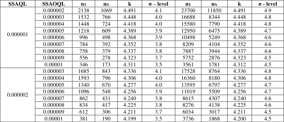 Table 1
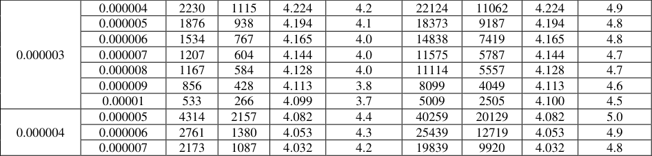 Table 1
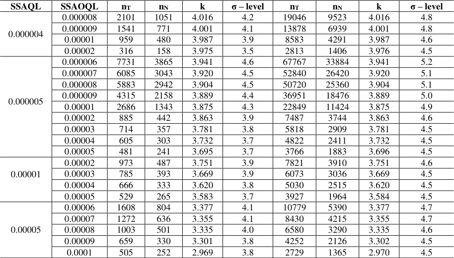 Table 1
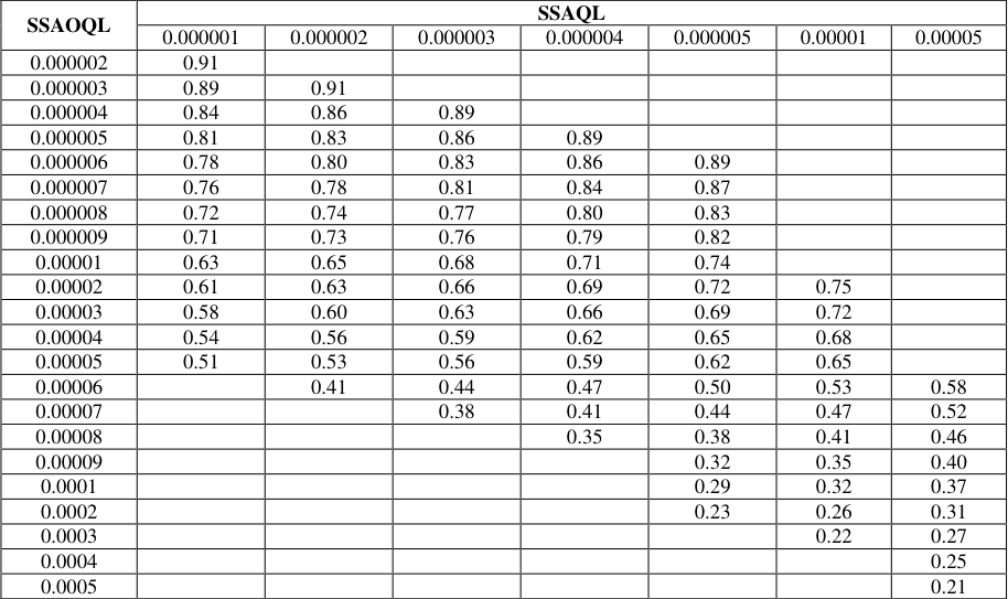 Table 2
Introduction
The designing procedure for the SSQSVSS (n Tσ , n Nσ ; k σ ) indexed by SSAQL and SSAOQL is based on Govindaraju (1990) [3] procedures and tables, developing for the selection of single sampling plan for variables indexed by AQL and AOQL. Soundararajan (1981) [9] has developed procedures and tables for the selection of single sampling plans for attributes for given AQL and AOQL. Govindaraju (1990) [3] has developed procedures and tables for the selection of single sampling plans for variables indexed by AQL and AOQL. Later Soundarajan and Palanivel (2000) [8] have developed procedures and tables for the selection of quick switching single sampling variables systems indexed by AQL and AOQL. Based on above article Senthilkumar and Esha Raffie (2017) [6] have constructed SSQSVSS (n σ ; k Tσ , k Nσ ) indexed by Six Sigma AQL and Six Sigma AOQL. The extension work of SSQSVSS (n Nσ , n Tσ ; k σ ) indexed by Six Sigma AQL and Six Sigma AOQL are given in this article. This concept can be extended to variable quality characteristics of the study, the resulting plan would be designated as SSQSVSS and would be applied under the following conditions: The production is steady, so that results on current and preceding lots are broadly indicative of a continuous process. Lots are submitted substantially in the order of production. Inspection is by variables, with the quality being defined as the fraction of nonconforming. The sample units are selected from a large lot and production is continuous. The production process should depend on automation and human handling is very negligible. The industry may adopt system method with decision makers having an experience in adopting the six sigma quality initiatives.
Basic Assumptions
The quality characteristic is represented by a random variable X measurable on a continuous scale. Distribution of X is normal with mean and standard deviation. An upper limit U, has been specified and a product is qualified as defective when X > U.
[when the lower limit L is Specified, the product is a defective one if X < L] The Purpose of inspection is to control the fraction defective, p in the lot inspected.
The condition for application above basic assumptions of SSQSVSS (n Tσ , n Nσ ; k σ ) system are the same as that of the SSQSVSS (n σ ; k Tσ , k Nσ ) system. The fraction defective in a lot will be p=
Where z ~ N (0, 1). Under the σmethod plan, the lot would be accepted if X + k σ U, ≤
where U is the upper specification limit or X + k σ L, ≥
where L is the lower specification limit.
Procedure of SSQSVSS (nTσ, nNσ; kσ) with known σ variables plan as the reference plan
The Six Sigma Quick Switching Variables Sampling System with known σ variables plan as the reference plan has following operating procedure
Operating procedure
Operating procedure
Step 4: i) If X + k σ U or X k σ L accept the lot and repeat Step 1, for the next lot.
ii) If X + k σ > U or X k σ < L, reject the lot and repeat Step 3.
Where n Nσ and n Tσ are the sample sizes of normal and tightened single sampling variable plans respectively, and k is the acceptance constant under σ-method. Where X and σ are the average quality characteristic and standard deviation respectively. The Six Sigma Quick Switching Variables Sampling System as SSQSVSS (n T , n N ; k σ ). As the tightened plan sample size n T is greater than the normal plan sample size n N , for designing the SSQSVS system n T is fixed as a multiple of n N i.e. n T = m n N , where m >1. Thus the QSS can also be designated as SSQSVSS (mn N , n N ; k σ ).
Based on Romboski (1969), the OC function of SSQSVSS (n Tσ , n Nσ ; k σ ) can be written as
The fraction nonconforming in a given lot has been given in (1) with v= (U-µ)/σ and its probability of acceptance will be
If the quality of the accepted lot is p and all defective units found in the rejected lots are replaced by non-defective units in a rectifying inspection plan, the Six Sigma average outgoing quality (SSAOQ) can be approximated as SSAOQ = pP a (p) (5) where P a (p) is defined in equation (2). If p m is the proportion nonconforming items at which SSAOQ is maximum, one has
If SSAQL (p 1 ) is prescribed, then the corresponding value of v SSAQL or v 1 will be fixed and if P a (p) is fixed at 99.99966%, that is (1-α). Where, α = 0.0000034x10 - 1 should understand the limitations of plans indexed by SSAOQL. Sampling with rectifying of rejected lots on the one hand reduces the average percentage of nonconforming items in the lots, but on the other hand introduces nonhomogeneity in the series of lots finally accepted. That is, any particular lot will have a quality of p% or 0% nonconforming depending on whether the lot is accepted or rectified. Thus the assumption underlying the SSAOQL principle is that the homogeneity in the qualities of individual lots is unimportant and only the average quality matters. For plans listed in Table 1, if the individual lot quality happens to be the product quality p m at which SSAOQL occurs, then the associated probability of acceptance will be poor. Table 2 gives P a (p m ) values of plans given in Table 1. For example, for SSAQL is 0.000004 and SSAOQL is 0.00001, Table 2 gives P a (p m ) = 0.71. Then p m = SSAOQL/ P a (p m ) = 0.000014. In order to avoid such inconvenience, the producer should maintain the process quality more or less at the SSAQL. The higher rate of rejection of lots at p = p m will also indirectly put pressure on the producer to improve the submitted quality.
| SSAOQL | SSAQL | — | — | — | — | — | — |
|---|---|---|---|---|---|---|---|
| 0.000001 | 0.000002 | 0.000003 | 0.000004 | 0.000005 | 0.00001 | 0.00005 | |
| 0.000002 | 0.91 | ||||||
| 0.000003 | 0.89 | 0.91 | |||||
| 0.000004 | 0.84 | 0.86 | 0.89 | ||||
| 0.000005 | 0.81 | 0.83 | 0.86 | 0.89 | |||
| 0.000006 | 0.78 | 0.80 | 0.83 | 0.86 | 0.89 | ||
| 0.000007 | 0.76 | 0.78 | 0.81 | 0.84 | 0.87 | ||
| 0.000008 | 0.72 | 0.74 | 0.77 | 0.80 | 0.83 | ||
| 0.000009 | 0.71 | 0.73 | 0.76 | 0.79 | 0.82 | ||
| 0.00001 | 0.63 | 0.65 | 0.68 | 0.71 | 0.74 | ||
| 0.00002 | 0.61 | 0.63 | 0.66 | 0.69 | 0.72 | 0.75 | |
| 0.00003 | 0.58 | 0.60 | 0.63 | 0.66 | 0.69 | 0.72 | |
| 0.00004 | 0.54 | 0.56 | 0.59 | 0.62 | 0.65 | 0.68 | |
| 0.00005 | 0.51 | 0.53 | 0.56 | 0.59 | 0.62 | 0.65 | |
| 0.00006 | 0.41 | 0.44 | 0.47 | 0.50 | 0.53 | 0.58 | |
| 0.00007 | 0.38 | 0.41 | 0.44 | 0.47 | 0.52 | ||
| 0.00008 | 0.35 | 0.38 | 0.41 | 0.46 | |||
| 0.00009 | 0.32 | 0.35 | 0.40 | ||||
| 0.0001 | 0.29 | 0.32 | 0.37 | ||||
| 0.0002 | 0.23 | 0.26 | 0.31 | ||||
| 0.0003 | 0.22 | 0.27 | |||||
| 0.0004 | 0.25 | ||||||
| 0.0005 | 0.21 |
Table text extracted from the original PDF; superscript letters are shown inline. The original table image is below.
View original table image
| SSAQL | SSAOQL | nT | nN | k | σ – level | nT | nN | k | σ – level |
|---|---|---|---|---|---|---|---|---|---|
| 0.000004 | 0.000008 | 2101 | 1051 | 4.016 | 4.2 | 19046 | 9523 | 4.016 | 4.8 |
| 0.000009 | 1541 | 771 | 4.001 | 4.1 | 13878 | 6939 | 4.001 | 4.8 | |
| 0.00001 | 959 | 480 | 3.987 | 3.9 | 8583 | 4291 | 3.987 | 4.6 | |
| 0.00002 | 316 | 158 | 3.975 | 3.5 | 2813 | 1406 | 3.976 | 4.5 | |
| 0.000005 | 0.000006 | 7731 | 3865 | 3.941 | 4.6 | 67767 | 33884 | 3.941 | 5.2 |
| 0.000007 | 6085 | 3043 | 3.920 | 4.5 | 52840 | 26420 | 3.920 | 5.1 | |
| 0.000008 | 5883 | 2942 | 3.904 | 4.5 | 50720 | 25360 | 3.904 | 5.1 | |
| 0.000009 | 4315 | 2158 | 3.889 | 4.4 | 36951 | 18476 | 3.889 | 5.0 | |
| 0.00001 | 2686 | 1343 | 3.875 | 4.3 | 22849 | 11424 | 3.875 | 4.9 | |
| 0.00002 | 885 | 442 | 3.863 | 3.9 | 7487 | 3744 | 3.863 | 4.6 | |
| 0.00003 | 714 | 357 | 3.781 | 3.8 | 5818 | 2909 | 3.781 | 4.5 | |
| 0.00004 | 605 | 303 | 3.732 | 3.7 | 4822 | 2411 | 3.732 | 4.5 | |
| 0.00005 | 481 | 241 | 3.695 | 3.7 | 3766 | 1883 | 3.696 | 4.5 | |
| 0.00001 | 0.00002 | 973 | 487 | 3.751 | 3.9 | 7821 | 3910 | 3.751 | 4.6 |
| 0.00003 | 785 | 393 | 3.669 | 3.9 | 6073 | 3036 | 3.669 | 4.5 | |
| 0.00004 | 666 | 333 | 3.620 | 3.8 | 5030 | 2515 | 3.620 | 4.5 | |
| 0.00005 | 529 | 265 | 3.583 | 3.7 | 3927 | 1964 | 3.584 | 4.5 | |
| 0.00005 | 0.00006 | 1608 | 804 | 3.377 | 4.1 | 10779 | 5390 | 3.377 | 4.7 |
| 0.00007 | 1272 | 636 | 3.355 | 4.1 | 8430 | 4215 | 3.355 | 4.7 | |
| 0.00008 | 1003 | 501 | 3.335 | 4.0 | 6580 | 3290 | 3.335 | 4.6 | |
| 0.00009 | 659 | 330 | 3.301 | 3.8 | 4252 | 2126 | 3.302 | 4.5 | |
| 0.0001 | 505 | 252 | 2.969 | 3.8 | 2729 | 1365 | 2.970 | 4.5 |
Table text extracted from the original PDF; superscript letters are shown inline. The original table image is below.
View original table image
| 0.000003 | 0.000004 | 2230 | 1115 | 4.224 | 4.2 | 22124 | 11062 | 4.224 | 4.9 |
|---|---|---|---|---|---|---|---|---|---|
| 0.000005 | 1876 | 938 | 4.194 | 4.1 | 18373 | 9187 | 4.194 | 4.8 | |
| 0.000006 | 1534 | 767 | 4.165 | 4.0 | 14838 | 7419 | 4.165 | 4.8 | |
| 0.000007 | 1207 | 604 | 4.144 | 4.0 | 11575 | 5787 | 4.144 | 4.7 | |
| 0.000008 | 1167 | 584 | 4.128 | 4.0 | 11114 | 5557 | 4.128 | 4.7 | |
| 0.000009 | 856 | 428 | 4.113 | 3.8 | 8099 | 4049 | 4.113 | 4.6 | |
| 0.00001 | 533 | 266 | 4.099 | 3.7 | 5009 | 2505 | 4.100 | 4.5 | |
| 0.000004 | 0.000005 | 4314 | 2157 | 4.082 | 4.4 | 40259 | 20129 | 4.082 | 5.0 |
| 0.000006 | 2761 | 1380 | 4.053 | 4.3 | 25439 | 12719 | 4.053 | 4.9 | |
| 0.000007 | 2173 | 1087 | 4.032 | 4.2 | 19839 | 9920 | 4.032 | 4.8 |
Table text extracted from the original PDF; superscript letters are shown inline. The original table image is below.
View original table image
| SSAQL | SSAOQL | nT | nN | k | σ – level | nT | nN | k | σ - level |
|---|---|---|---|---|---|---|---|---|---|
| 0.000001 | 0.000002 | 2138 | 1069 | 4.491 | 4.1 | 23700 | 11850 | 4.491 | 4.9 |
| 0.000003 | 1532 | 766 | 4.448 | 4.0 | 16688 | 8344 | 4.448 | 4.8 | |
| 0.000004 | 1448 | 724 | 4.418 | 4.0 | 15580 | 7790 | 4.418 | 4.8 | |
| 0.000005 | 1218 | 609 | 4.389 | 3.9 | 12950 | 6475 | 4.389 | 4.7 | |
| 0.000006 | 996 | 498 | 4.368 | 3.9 | 10498 | 5249 | 4.368 | 4.6 | |
| 0.000007 | 784 | 392 | 4.352 | 3.8 | 8209 | 4104 | 4.352 | 4.6 | |
| 0.000008 | 758 | 379 | 4.337 | 3.8 | 7887 | 3944 | 4.337 | 4.6 | |
| 0.000009 | 556 | 278 | 4.323 | 3.7 | 5752 | 2876 | 4.323 | 4.5 | |
| 0.00001 | 346 | 173 | 4.311 | 3.5 | 3561 | 1781 | 4.312 | 4.5 | |
| 0.000002 | 0.000003 | 1685 | 843 | 4.336 | 4.1 | 17528 | 8764 | 4.336 | 4.8 |
| 0.000004 | 1593 | 796 | 4.306 | 4.0 | 16360 | 8180 | 4.306 | 4.8 | |
| 0.000005 | 1340 | 670 | 4.277 | 4.0 | 13595 | 6797 | 4.277 | 4.7 | |
| 0.000006 | 1096 | 548 | 4.256 | 3.9 | 11019 | 5509 | 4.256 | 4.7 | |
| 0.000007 | 862 | 431 | 4.240 | 3.8 | 8615 | 4307 | 4.240 | 4.6 | |
| 0.000008 | 834 | 417 | 4.225 | 3.8 | 8276 | 4138 | 4.225 | 4.6 | |
| 0.000009 | 612 | 306 | 4.211 | 3.7 | 6034 | 3017 | 4.211 | 4.5 | |
| 0.00001 | 381 | 190 | 4.199 | 3.5 | 3736 | 1868 | 4.200 | 4.5 |
Table text extracted from the original PDF; superscript letters are shown inline. The original table image is below.
View original table image
Procedure of unknown σ SSQSVSS for given SSAQL and SSLQL
If the population standard deviation σ is unknown, then it is estimated from the sample standard deviation S (n-1 as the divisor). If the sample size of the unknown sigma variables system (S-method) is n Ts , n Ns and the acceptance constant is k s , then the operating procedure is as follows
Step 1: Draw a sample of size n s from the lot, inspect and record the measurement of the quality characteristic for each unit of the sample. Compute the sample mean X and sample standard deviation S N .
Selection of unknown σ SSQSVSS (nTs, nNs; ks) for Given SSAQL and SSAOQL
Table 1 also gives such matched s-method plan. For example, for given SSAQL is 0.00001 and SSAOQL is 0.00004, one obtains the parameters of the s-method plan from Table 1 to be n Ts = 5030, n Ns = 2515 and k s = 3.620, which is associated with 4.5 sigma level of SSQSVSS (n Ts, n Ns ; k s ). The sample size n Ts = m n Ns = (2) (2515) = 5030. Thus, for the requirem-ent, the SSQSVSS (n Ts, n Ns ; k s ) id specified by the parameters, n Ts = 5030, n Ns = 2515 and k s = 3.620.
Construction of Table 1
For constructing Table 1, a trial value of p m is assumed and the probability of acceptance at p m is found using (6) as P a (p m ) = SSAOQL / p m (7) The auxiliary variables v m , w Nm and w Tm corresponding to the values of p m and P a (p m ) respectively, are found using (1), ( 2), ( 3) and ( 4). For given values of (p 1 , α), determine the values of v 1 , w N1 and w T1 using the approximation (Abramwitz and Stegun (1972)) for the ordinate of the cumulative normal distribution. With the values of v m , w Nm and w Tm , the following equation is used for calculating n Nσ . Equation ( 8) is the formula for finding the sample size of a known σ SSQSVS system. With the values of n obtained from (14), it is then checked to see whether the assumed value of p m corresponds to the proportion non-conforming at which the SSAOQL occurs or not. That is, it is checked to see whether or not the trial value of p m satisfies the following condition.
Equation ( 8) was obtained from the following relation
If the assumed value of p m does not satisfy (10), then another trial value of p m is obtained from (10) by numerical methods. The methods of successive substation is often found to give good results and ( 10) is rewritten for this purpose as
After determining the next trial value of p m , again the values of v m , w Nm , w Tm and n σ are found and the condition (14) rechecked. This iterative procedure continues until the convergence of p m is achieved. Then the value of k σ is obtained from (3) and (4).
For obtaining the values of v 1 , w N and w T , the approximation for the ordinate of the cumulative normal distribution available in Abramowitz and Stegun (1972) was used. The S-method plans matching the σ-method plans were obtained using computer search routine through C++ programme. For selected combinations of SSAQL and SSAOQL, Table 1 was constructed following the above iterative procedure.
The iterative procedure given above may also be used to determine a Six Sigma Quick Switching Sampling System for given Six Sigma Indifference Quality Level (SSIQL) and SSAOQL as well as for given Six Sigma Limiting Quality Level(SSLQL) and SSAOQL with appropriate auxiliary variables v, w N and w T .
References
9 in the original paper- Abramowitz M, Stegun IA. Handbook of Mathematical functions, Dover Publications, New York, 1972.
- Dodge HF. A New Dual System of Acceptance Sampling Technical Report, No.16, The Statistics Center, Rutgers-The State University, New Brunswick, NJ, 1967.
- Govindaraju K. Single sampling Plans for Variables Indexed by AQL and AOQL, Journal of Quality Technology. 1990; 22(4):310-313.
- Romboski LD. An Investigation of Quick Switching Acceptance Sampling Systems, Doctoral Dissertation, Rutgers the State University, New Brunswick, New Jersey, 1969.
- Senthilkumar D, Esha Raffie B. Six Sigma Quick Switching Variables Sampling System Indexed by Six Sigma Quality Levels, International Journal of Computer Science & Engineering Technology. 2012; 3(12):565-576.
- Senthilkumar D, Esha Raffie B. Quick Switching Variables Sampling System Indexed by Six Sigma AQL and Six Sigma AOQL, International Journal of Current Research in Science and Technology. 2017; 3(10):21-28.
- Sommers DJ. Two-point double variables sampling plans, Journal of Quality Technology, 1981, 13.
- Soundarajan V, Palanivel M. Quick Switching Variables Single Sampling (QSVSS) System indexed by AQL and AOQL, Journal of Applied Statistics. 2000; 27(7):771-778.
- Soundararajan V. Single Sampling Attributes Plans Indexed by AQL and AOQL, Journal of Quality Technology. 1981; 13(3):195-200.