Backward model building for nonparametric discrimination and classification of fatty liver cases

A backward-model-building algorithm for discrimination of two populations in a nonparametric setting has been recently proposed by Padmanaban and William (2016a). This approach is applicable without assumptions unlike the traditional approaches of constructing discriminant models. As an application of this approach, we consider the discrimination and classification of fatty-liver cases from non-fatty-liver cases through some observable variables that are generally thought of as factors associated with the health of the liver. The discriminant model is developed with a sample of 160 cases drawn from a case-control study. The resulting discriminant model is compared to binary logistic regression modelvis-a-vis discriminatory capacity as measured by Kolmogorov-Smirnov Statistic.

Illustrations explain the paper; they do not show study data.

AI-generated illustration

↗ Enlarge

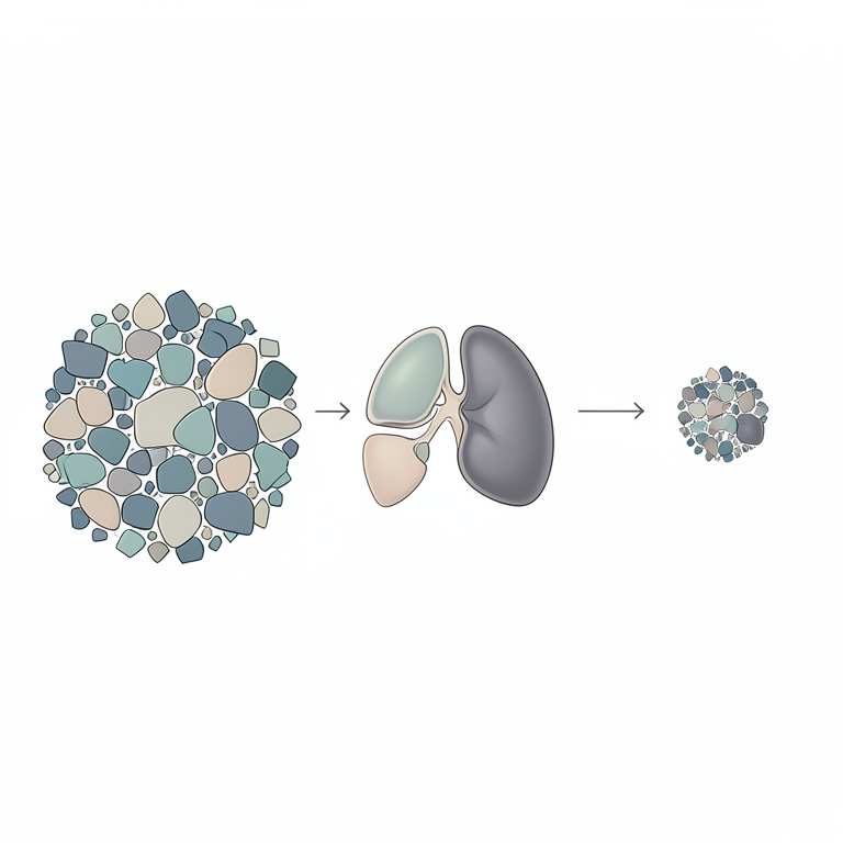
Backward Model-Building ProcessClose ×

AI-generated conceptual illustration (human liver tissue with steatosis). It explains the idea and does not show study data.

Open full-size image ↗

Introduction

Discriminant Analysis and the consequential issue of effectively classifying objects to the populations have remained an interesting problem of investigation over the past many years. However, in the context of classification / prediction involving two populations, binary logistic regression has become a preferred approach in recent times, as the 'restrictive assumptions' involved in Discriminant Analysis are not imposed in logistic regression. For the twopopulation situation, an approach followed to include or exclude variables from the discriminant is a comparison of means of the variables in the two populations. Also, the distance of the discriminant value from the average discriminant values in the two populations is taken as a criterion for classifying of an object to one of the two populations. Application of Discriminant Analysis in a non-parametric setting requires the variancecovariance matrices of the two populations to be equal, though this is not required for multivariate normal populations. In many applications, the conditions of multivariate normality or equality of variance-covariance matrices are not satisfied. For the case of multivariate normal populations, the equality of variance-covariance matrices can be tested and according to the conclusion, different approaches to discriminant analysis are adopted. For non-normal cases, there is no easy test available and so, practitioners generally assume the variance-covariance matrices as equal and proceed. Thus, there is a gap between theory and practice that has remained unaddressed so far. Discriminant Analysis has seen good theoretical and methodological developments in the past. The construction of discriminant models requires the identification of the important variables and elimination of those that are immaterial in discriminating the populations. An interesting early work in this context is a paper by Chang (1983) [5] wherein the separation of a mixture of two multivariate normal populations was taken up through principal components. In Bensmail and Celeux (1996) [3] , Gaussian discriminant analysis was addressed via eigen-value decomposition. Recently, Murphy et al. (2010) [11] proposed a stepwise algorithm that uses the 'Bayesian Information Criterion' following a similar approach suggested by Raftery and Dean (2006) [17] for model-based clustering. These papers focus on parametric settings and their scope for applications is restricted.

Discriminant analysis under non-parametric settings has been another direction of research pursued by various authors. Hastie et al. (1994) [8] considered nonparametric discriminant analysis with nonlinear classifiers to handle situations with a large number of input variables. Non-linear discriminant analysis via kernel approach, which is theoretically close to support vector machines, was provided by Baudat and Anouar (2000) [1] . Bressan and Vitria (2003) [4] developed nonparametric discriminant analysis with adaptation to nearest-neighbour classification. Chiang and Pell (2004) [6] combined genetic algorithms with discriminant analysis for identifying key variables. In all these papers, the focus has been on identification of the important variables that effectively discriminate the populations. Recently, Padmanaban and William (2016, 2016a) [12] proposed a discriminant analysis procedure with the required theoretical framework for a distribution-free setting which does not require the variance-covariance matrices to be equal. In these papers, a different approach has been taken for twopopulation discriminant analysis while adhering to the spirit and objective of classical discriminant analysis. We refer to these papers for the 'model performance measure' considered by the authors to assess the classification ability of discriminant models and the corresponding decision rule for locating the optimal cut-off point for classification. Also, Padmanaban and William (2016) [12] introduced a 'forwardmodel-building algorithm' for selecting the important variables from a set of candidate variables. In the same spirit, Padmanaban and William (2016a) [12] , proposed a 'backwardmodel-building algorithm' for eliminating the variables that are immaterial for discriminating the populations. This paper has four sections including this introduction section and is organized as follows: In Section 2, we review the basic theoretical framework, optimal discriminant function, model performance measure and the variableelimination (backward) algorithm to build an efficient discriminant model, which have been introduced by the authors recently. Section 3 discusses the phenomenon of fatty liver, a major health issue currently, and the factors believed to be associated with the phenomenon. In Section 4, as an application of the variable-elimination algorithm, we consider the classification and discrimination of fatty liver cases from others using measurements on eight observable variables using a sample of 160 cases drawn from a case-control study. We shall also compare the discriminant model performance with that of logistic regression.

A Review of the Recently Introduced Procedure

Let π1 and π2 be two populations with relative sizes in the proportions p1 and p2 respectively. The problem under consideration is the discrimination of the members of the two populations using observations on a random vector, say, X = (X1, X2, Xp) T . Let the mean-vectors of X in the two populations be μ1 = E1(X) and μ2 = E2(X) and the variancecovariance matrices of X be Σ1 and Σ2. Then we have the following results from Padmanaban and William (2016) [12] : (i) For a random vector X and another random object W, the relationship between the unconditional and conditional mean vectors and variance-covariance matrices is given by E(X) = EW[EX|W (X)] and V(X) = EW{VX|W(X)} + VW{ EX|W(X)} (2.1) (ii) The overall variance-covariance matrix of the combined population is given by Σ

3) If X(s) be a subset of the variables, then with similar notations, the X(s)-based optimal discriminant is Y(s)= (μ1(s) -μ2(s)) T Σ(s) -1 X(s)

(2.4) Typically, the parameters are replaced by the sample estimates in practice. The performance of the X(s)-based optimal discriminant is measured by the two sample Kolmogorov-Smirnov Statistic based on the Y(s) measurements given by

where R1(s)(•) and R2(s)(•) are the (empirical) reliability functions of Y(s) for the two populations. Given two subvectors X(s1) and X(s2), the optimal X(s1)-based discriminant is said to be 'more efficient' than the optimal X(s2)-based discriminant if KS(s1)> KS(s2). If there exists a random subvector X(s*) for which KS(s*)> KS(s) for every other random subvector X(s), then the corresponding optimal discriminant Y(s*) is the 'most efficient' discriminant. Finding the 'most efficient' discriminant is computationally prohibitive when there are a large number of variables. So, different algorithms are suggested to 'build' improved models in a sequential manner rather than finding the 'best' from 'all possible' models. Padmanaban and William (2016a) [12] developed a 'backward model-building' algorithm to build a 'sequence' of models, starting with 'all' variables and 'eliminate' variables one-by-one based on their 'irrelevance' in adding to the discriminatory capability of the model. The sequence of steps involved in the algorithm is briefly presented below: Let X1, X2, . . , Xp be the candidate input variables.

Step 0: Using all the candidate variables X, the X-based discriminant scores are computed for each individual record in the data. Let the value of the KS Statistic for this 'full' model be denoted KS(0). The significance of this statistic is evaluated at a desired level of significance.

Step 1: Removing one variable at a time, 'p' discriminants Y(~1), Y(~2), . . ., Y(~p), (where Y(~i) is the discriminant based on all variables except Xi), and their corresponding scores are obtained for each record in the data. Let the KS Statistic for Y(~i) be denoted as KS(~i). If KS(~i)> KS(~j) for every j ≠ i and KS(~i) ≥ KS(0) then among all the variables, Xi is the least effective discriminator between the two populations. So at the end of Step 1, Xi gets eliminated. In contrast, if KS(~i)> KS(~j) for every j ≠ i but KS(~i)<KS(0) then Xi does not leave the model, nor any of the remaining Xj's leave as theirexit leads to reduced discriminatory ability and the model building stops with all the 'p' candidate variables present.

Step 2: If Xi were eliminated in Step 1, we remove one additional variable at a time and obtain (p-1) discriminants, in which the removed variables are (X1,Xi), . . . . , (Xi-1,Xi), (Xi+1,Xi),....,(Xp,Xi). Denote the discriminants as Y( ,i), Y(~2!.i),..., Y(~i-1,~i), Y(~i+1,~i), ... Y(~p,~i) and the corresponding Kolmogorov-Smirnov statistics as KS( ,i), KS(~2,~i),...,KS(~i-1,~i), KS(~i+1,~i),..., KS(~p,~i). If for some 'm', KS(~m~,i)> KS(~j~,i) for every j ≠ m, and KS(~m,~i) ≥ KS(~i), then Xm leaves the model in Step 2. In contrast, if KS(~m,~i)> KS(~j,~i) for every j ≠ m, but KS(~m,~i) < KS(~i), then Xm does not leave the model, nor any of the remaining Xj's leave, as their exit leads to reduced discriminatory ability and the model building stops with (p -1) input variables present. Clearly no other variable can leave further. At every step, one more variable leaves if the maximum KS value at that step exceeds or equals the maximum KS value of the previous step. If it is less than the previous maximum, the process stops. When the process stops at the (k+1) th step, the efficient discriminant function is the one obtained in the k th step with the maximum KS value, leading to significant and maximum discrimination between the two populations. We denote the final subset of variables remaining (without getting eliminated) in this process as X(S*) and the 'final' efficient discriminant as Y(s*). The 'explanation' to the KS statistic and also the suggestion to use the 'survival Function' for computing the KS Statistic are provided in the paper of Padmanaban and William (2016) [12] wherein the proposal for forward model-building process was initially given before the backward process of Padmanaban and William (2016a) [12] .

Classification or prediction rule

The classification or prediction rule to classify an individual object to one of the two populations is based on the optimal cut point at which the KS statistic value is attained. Let y0 be the point such that

The phenomenon of non-alcoholic fatty-liver disease Overview

Non-alcoholic fatty liver disease (NAFLD) is a condition where there is excess accumulation of fat in the liver of people who drink little or no alcohol. The most common form of NAFLD is a non-serious condition known as fatty liver. When fat accumulates in the liver cells, it becomes fatty liver. Fat accumulation in the liver is not normal, but by itself it probably does not damage the liver. A small group of people with NAFLD may have a serious condition known as non-alcoholic steatohepatitis (NASH). Sayiner et. al. (2016) [15] report a study on the epidemiology of NAFLD and NASH in the United States and the rest of the world. In NASH, fat accumulation leads to liver cell inflammation and different degrees of scarring. NASH is a potentially serious condition and may lead to severe liver scarring and cirrhosis. Cirrhosis occurs when the liver suffers significant damage, and the liver cells are gradually replaced by scar tissue, affecting the ability of the liver to function well. Sometimes liver transplant may be needed on patients who develop cirrhosis. We refer to Benedict and Zhang (2017) [2] for an expanded review of NAFLD.

Incidence

Non-alcoholic fatty liver disease (NAFLD) is a distinct hepatic condition and one of the most common causes of chronic liver disease. Prevalence of the disease is estimated to vary from 9% to 32% in the Indian population, with higher incidence rate amongst obese and diabetic patients.For more details in the Indian context we refer to Kalra et al. (2013) [10] . A similar study on people of different races and ethnicities has been reported in Kalia and Gaglio (2016) [9] .

Methodology

The patients attending gastroenterology out-patient department and confirmed as fatty liver cases are selected as the study group. Those patients diagnosed as not having fatty liver are selected as control group. A sample of 80 from each group has been included for this study.

Potential Factors Associated with Fatty liver

(1) AGE -A common perception is that older a person, higher is the possibility for diseases affecting the inner organs including fatty liver condition. ( 2) TRIGLYCERIDE (mg/dl) -Elevated TGL is observed in obese people, diabetics and people who consume alcohol and is associated with heart and blood vessel disease. (3) GGT (U/L) -The gamma-glutamyl transferase test may be used to determine the level of alkaline phosphatase (ALP) which is likely to indicate liver disease. ( 4) HEIGHT (cm) -Although Height has no direct or causative relationship to the condition of inner organs, it being a variable used to measure BMI makes it a candidate variable. ( 5) WEIGHT (kg) -Weight increase is associated with lifestyle diseases and with liver diseases too. (6) BMI -Body mass index is an indicator of an individual's health and could be associated with fatty liver. (7) WAIST CIRCUMFERENCE (cms) -The waistline is generally considered to be another indicator of the health of a person, and probably indicates the condition of one's liver. (8) FLI -The Fatty Liver Index is based on Waist Circumference, Body Mass Index, Triglyceride and GGT and was initially developed to detect fatty liver.

Objective: This study aims to relate the above factors to fatty liver through the backward model building approach of nonparametric discriminant analysis developed by Padmanabanand William (2016a) [12] . We wish to identify the important factors associated with fatty liver and also give a decision rule to classify people as 'fatty liver cases' or not. We apply the backward-model-building algorithm developed in this paper and get the following results.

Step 0: The KS statistic for the model with all eight variables is found to beKS(0) = 0.675

Step 1: The KS statistics for models with elimination of one variable are: KS(~X1) = 0.55, KS(~X2) = 0.625, KS(~X3) = 0.5625, KS(~X4) = 0.6125, KS(~X5) = 0.6375, KS(~X6) = 0.6125, KS(~X7) = 0. We observe from (4.1) that, higher age, higher TGL, higher GGT and larger waist circumference all indicate higher likelihood for the individual to have fatty liver. Such an explanation is not possible individually for height, weight, BMI and FLI but all these collectively represent the obesity / overweight factor which is bad for health in general. In fact FLI is based on Waist Circumference, Body Mass Index, Triglyceride and GGT and the inclusion of FLI along with these variables does not ensure an expected sign for its coefficient (like the collinearity situation in regression models). However, for predictive purposes, we do not insist on only intuitive signs for variables that are entangled in collinear relationships. The ultimate objective is efficient classification.

Comparison with Logistic Regression Model

Denoting 'fatty liver presence' as the outcome of interest, we build a logistic regression model using the backward stepwise method:

Step 1: (With all eight variables) where 'p' is the probability for 'Fatty Liver presence'. The KS for this model is found to be 0.6625 which is less than the KS obtained for the 'Efficient Discriminant Model' (4.1). Thus, the predictive performance of our method is superior to that of binary logistic regression method in predicting fatty liver cases. It is interesting to note that, while the backward stepwise logistic regression removes 'Weight' and retains the remaining seven variables under consideration, our discriminant model includes Weight also additionally. Although, BMI along with 'Height' indirectly captures the effect of 'Weight' and therefore, removed in the logistic regression algorithm, our backward stepwise discriminant modelling algorithm retains 'Weight' additionally. We wish to highlight that, though the new approach needs to be applied to many more situations involving binary outcome variables to study its effectiveness, the present findings point out that this approach is a promising alternative to logistic regression. It is also observed that this approach is capable of discovering some important discriminators which logistic regression approach fails to identify.

Figures and tables from the paper

Fatty liver	AGE	TGL(mg/dl)	GGT(U/L)	HEIGHT(cms)	WEIGHT(KG)	BMI	WAIST (cms)	FLI
1	54	125	58	144	62.7	30.2	91	68.8385268
2	32	130	27	158	60	24.03	102	50.1745485
2	43	102	45	158	60	24	90	37.7959715
1	22	52	15	148	63	28.8	108	42.3631145
1	50	220	45	152	68	29.4	112	89.5753849

Table text extracted from the original PDF; superscript letters are shown inline. The original table image is below.

View original table image

↗ Enlarge

Table 1Close ×

A sample of the data on the eight variables listed under 'Potential indicators' along with the birth outcome (Fatty liver = 1, No Fatty

Open full-size image ↗

Original paper tableSource PDF · page 4 ↗

1. Baudat G, Anouar F. Generalized Discriminant Analysis using a Kernel Approach. Neural Computation, 2000; 12(10):2385-2404.
2. Benedict M, Zhang X. Non-alcoholic fatty liver disease: An expanded review. World J. Hepatol. 2017; 9:715-732.
3. Bensmail H, Celeux G. Regularized Gaussian discriminant analysis through eigen value decomposition. J. Amer. Statist. Assoc. 1996; 91:1743-1748.
4. Bressan M, Vitria J. Nonparametric Discriminant Analysis and Nearest Neighbor Classification. Pattern Recognition Letters. 2003; 24:2743-2749.
5. Chang WC. On using Principal Components before Separating a Mixture of two Multivariate Normal Distributions J. Roy. Statist. Soc. Ser C. 1983; 32:267275.
6. Chiang LH, Pell RJ. Genetic algorithms combined with discriminant analysis for key variable identification. J. Process Control, 2004; 14:143-155.
7. Habbema JDF, Hermans J. Selection of variables in discriminant analysis by F-Statisticand error rate. Technometrics. 1977; 19:487-493.
8. Hastie T, Tibshirani R, Buja A. Flexible Discriminant Analysis by Optimal Scoring. Amer. Statist. Assoc. 1994; 89:1255-1270.
9. Kalia HS, Gaglio PJ. The Prevalence and Pathobiology of Nonalcoholic Fatty Liver Disease in Patients of Different races or Ethnicities. Clin. Liver Dis. 2016; 20:215-224.
10. Kalra S, Vithalani M, Gulati G, Kulkarni CM, Kadam Y, Pallivathukkal J, et al. Study of prevalence of nonalcoholic fatty liver disease (NAFLD) in type 2 diabetes patients in India (SPRINT). J. Assoc. Physicians India, 2013; 61:448-453.
11. Murphy TB, Dean N, Raftery AE. Variable Selection and updating in Model-Based Discriminant Analysis for High Dimensional Data with Food Authenticity Applications. The Annals of Applied Statistics, 2010; 4(1):396-421.
12. Padmanaban S, Martin L. William. A nonparametric discriminant variable-selection algorithm for classification to two populations International Journal of Applied Mathematics and Statistical Sciences. 2016; 5(2):87-98.
13. Pfeiffer KP. Stepwise Variable Selection and Maximum Likelihood Estimation of Smoothing Factors of Kernel Functions for Nonparametric Discriminant Functions evaluated by Different Criteria. J. Biomed. Informatics. 1985; 18:46-61.
14. Raftery AE, Dean N. Variable Selection for Model-Based Clustering. J. Amer. Statist Assoc. 2006; 101:168-178.
15. Sayiner M, Koenig A, Henry L, Younossi ZM. Epidemiology of Nonalcoholic Fatty Liver Disease and Nonalcoholic Steatohepatitis in the United States and the Rest of the World. Clin. Liver Dis., 2016; 20:205-214.