
Research article · 2018 · Full text
International Journal of Statistics and Applied MathematicsStatistical properties and applications of a Weibull-Kumaraswamy distribution
Volume 3(6) · Pages 80–90
Research areasStatistical Distribution Estimation and ApplicationsHydrology and Drought AnalysisAgricultural Economics and Practices
Abstract
Author-writtenThe Kumaraswamy probability distribution was originally proposed by Poondi Kumaraswamy (1980) for double bounded random processes for hydrological applications. Here, we proposed a new extension of the Kumaraswamy distribution by adding one shape and one scale parameter to the Kumaraswamy distribution using the Weibull link function proposed by Tahir et al. (2015). This study has derived some expressions for its basic statistical properties such as moments, moment generating function, the characteristics function, reliability analysis, quantile function and the distribution of order statistics. Some plots of the distribution and the reliability function were generated and interpreted appropriately. The model parameters have been estimated using the method of maximum likelihood estimation. The performance of the Weibull-Kumaraswamy distribution has also been tested by some applications to two real data sets.
Summary
Source-checkedPlain-language reading of the full paper, prepared with AI and checked against the text. Each point links to the authors' own words.
Why it matters
- The Kumaraswamy distribution was first created for hydrological applications involving random processes that are double bounded. View evidence ↗
- Researchers use generalized families of distributions to create compound distributions, which often provide better performance than the original distributions. View evidence ↗
The question
- The authors aim to introduce a new extension of the Kumaraswamy distribution, called the Weibull-Kumaraswamy distribution (WKD), by adding a scale and a shape parameter via a Weibull link function. View evidence ↗
What they did
- The study derives several mathematical expressions for the WKD, including its moments, moment generating function, characteristics function, quantile function, and order statistics. View evidence ↗
- The authors used the method of maximum likelihood estimation (MLE) to estimate the parameters of the proposed model. View evidence ↗
- The WKD was tested using two real-world datasets: flood data with 20 observations and rock sample shape measurements with 48 observations. View evidence ↗
What they found
- The WKD is flexible in its shape, capable of being either left-skewed or right-skewed depending on the chosen parameter values. View evidence ↗
- Reliability analysis shows that the survival probability of a variable following the WKD decreases as the variable's value (or age) increases. View evidence ↗
- The hazard function analysis indicates that the probability of failure for the WKD increases as time or age increases. View evidence ↗
- For Data set I, the WKD was ranked as the best model (Rank 1) with an AIC of -23.9569 and a BIC of -19.9739. View evidence ↗
- For Data set II, the WKD again performed best (Rank 1), showing an AIC of -107.7825 and a BIC of -100.2977. View evidence ↗
- The WKD outperformed the Kumaraswamy-Kumaraswamy (KKD), Exponentiated Kumaraswamy (EKD), Transmuted Kumaraswamy (TKD), and the classical Kumaraswamy (KD) distributions across both datasets. View evidence ↗
What it means
- The authors conclude that the WKD is suitable for modeling events dependent on time or age where the survival rate declines over time. View evidence ↗
- The authors state that the WKD provides a superior fit compared to several other generalizations of the Kumaraswamy distribution. View evidence ↗
Visual summary
3 visualsIllustrations explain the paper; charts are replotted from the paper's own table values.
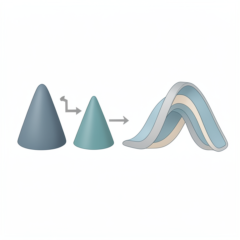
Conceptual Construction of WKD
AI-generated conceptual illustration (Abstract geometric representations of probability density functions). It explains the idea and does not show study data.
View source evidence ↗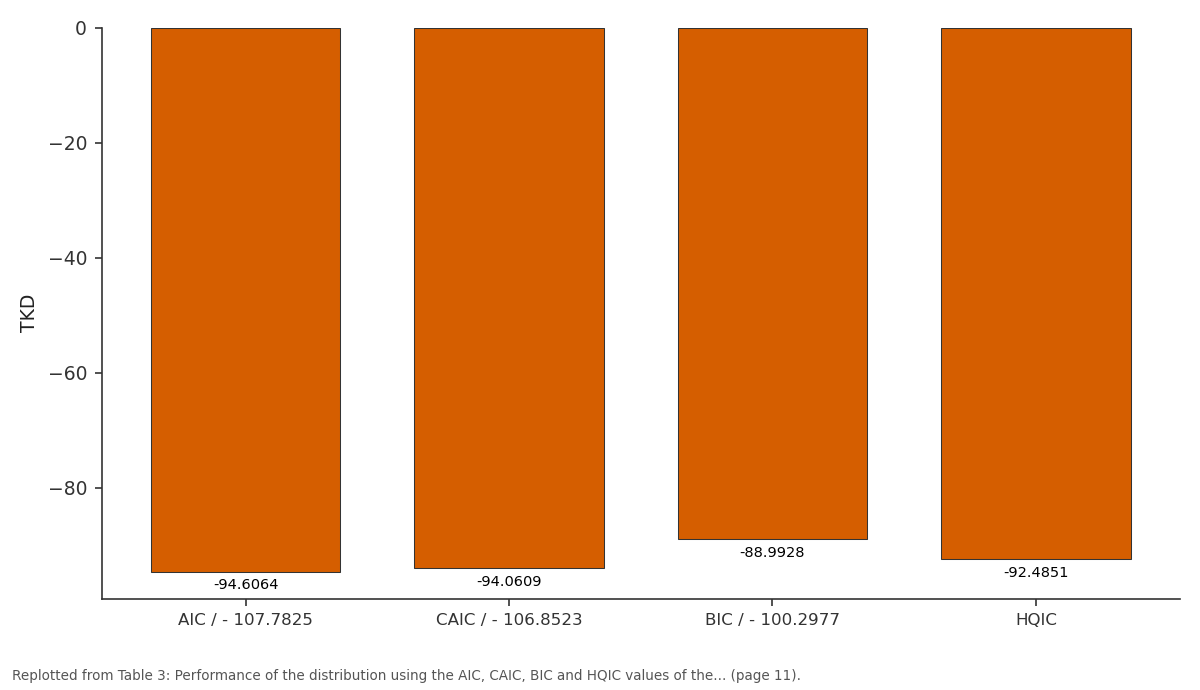
TKD: AIC / - 107.7825 vs CAIC / - 106.8523 vs BIC / - 100.2977 vs HQIC
Replotted from Table 3 (page 11) of the original paper. Every bar is the paper's own table value.
View source evidence ↗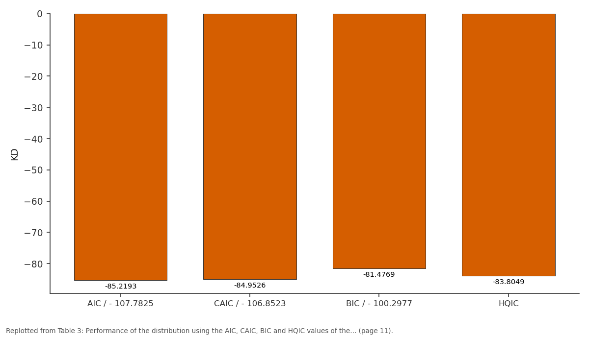
KD: AIC / - 107.7825 vs CAIC / - 106.8523 vs BIC / - 100.2977 vs HQIC
Replotted from Table 3 (page 11) of the original paper. Every bar is the paper's own table value.
View source evidence ↗Figures & tables
From the original paper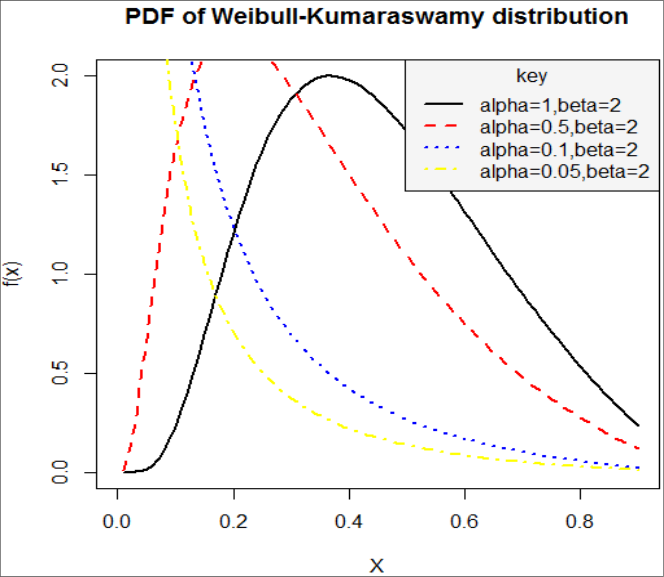 Fig. 1
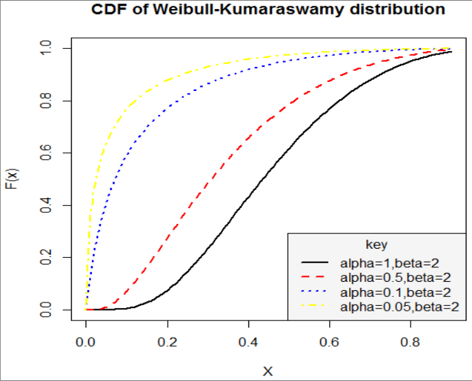 Figure 2
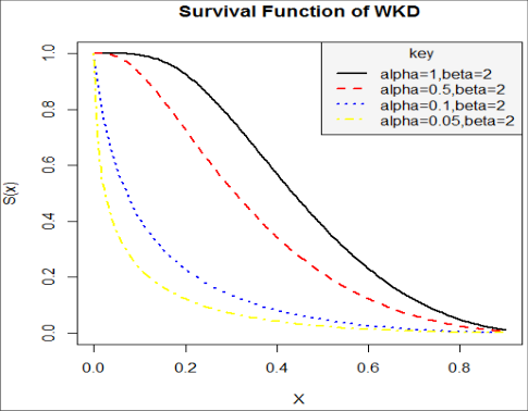 Figure 3
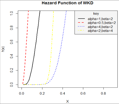 Figure 4
 Table 1
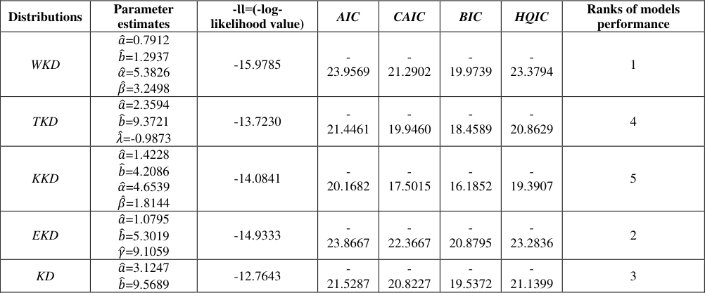 Table 2
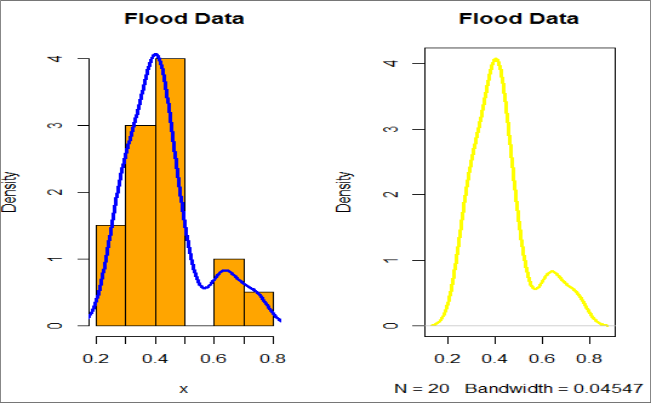 Figure 5
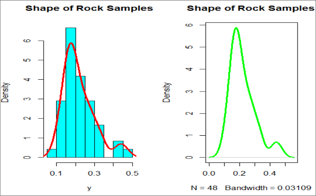 Figure 6
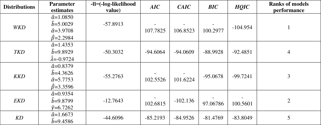 Table 3
Introduction
The Kumaraswamy probability distribution was originally proposed by Poondi Kumaraswamy (1980) [6] for double bounded random processes for hydrological applications. The Kumaraswamy double bounded distribution denoted by (a, b) distribution is a family of continuous probability distributions defined on the interval [0, 1] with cumulative distribution function (cdf) given by (1) And the corresponding probability density function (pdf) given by (2) For
, where a> 0 and b> 0 are the shape parameters. We have so many generalized families of distributions proposed by different researchers that are used in extending other distributions to produce compound distributions with better performance. We also have some generalizations of the Kumaraswamy distribution recently proposed in the literature such as the transmuted Kumaraswamy distribution by Khan et al., (2016) [5] , the exponentiated Kumaraswamy distribution by Javanshiri et al. (2015) [3] and the Kumaraswamy-Kumaraswamy distribution by El-Sherpieny and Ahmad (2014) [2] . In the next section, we have obtained the cdf and pdf of the Weibull-Kumaraswamy distribution (WKD) using the steps proposed by Tahir et al, (2015) [7] . According to them, the formula for deriving the cdf and pdf of any Weibull-based distribution from the above Weibull-G family is defined for any continuous distribution as follows:
Respectively, where g(x) and G(x) are the pdf and cdf of any continuous distribution to be generalized respectively and 𝛼>0 and β>0 are the two additional new parameters responsible for the scale and shape of the distribution respectively. The aim of this article is to introduce a new continuous distribution called Weibull-Kumaraswamy distribution (WKD) from the proposed family by Tahir et al. (2015) [7] . The remaining parts of this paper are presented in sections as follows: We defined the new distribution and give its plots in section 2. Section 3 derived some properties of the new distribution. The estimation of parameters using maximum likelihood estimation (MLE) is provided in section 4. In section 5, we carryout application of the proposed model with others to two real life data sets. Lastly, in section 6, we give some concluding remarks.
The Weibull-Kumaraswamy distribution (WKD)
Using equation ( 1) and ( 2) in ( 3) and ( 4) and simplifying, we obtain the cdf and pdf of the Weibull-Kumaraswamy distribution as follows:
(5) and ( 6) respectively.
For
, where a> 0 and b> 0 are the shape parameters while are scale and shape parameters respectively. Given some values for the parameters α, β, a and b, we provide some possible shapes for the pdf and the cdf of the WKD as shown in figure 1 and 2 below: From the above cdf plot, the cdf increases when X increases, and approaches 1 when X becomes large, as expected.
Properties
In this section, we defined and discuss some properties of the WKD distribution.
Moments
Let X denote a continuous random variable, the n th moment of X is given by;
Considering f(x) to be the pdf of the Weibull-Kumaraswamy distribution as given in equation (7).
Let
Then, using a power series expansion for A, we can write A as:
Substituting for the expansion above in equation ( 8), we have;
Also, let then, the following formula holds for B for i≥1 (http://function.wolfram.com/Elementaryfunctions/log/06/01/04/03/), and then we can write the B as follows:
Where for (for j≥0) P j,0 =1 and (for k=1,2,…..)
Combining equation ( 9) and inserting the above power series in equation ( 10) and simplifying, we have:
Now, if l is a positive non-integer, we can expand the last term in (12) as:
Recall the for the Kumaraswamy distribution;
Hence, this implies that (15)
The Mean
The mean of the WKD can be obtained from the n th moment of the distribution when n=1 as follows:
Also the second moment of the WKD is obtained from the n th moment of the distribution when n=2 as (17)
The Variance
The n th central moment or moment about the mean of X, say 𝜇 𝑛 , can be obtained as
The variance of X for WKD is obtained from the central moment when n=2, that is,
The variation, skewness and kurtosis measures can also be calculated from the non-central moments using some well-known relationships.
Moment Generating Function
The mgf of a random variable X can be obtained by (21)
Using power series expansion in equation ( 21) and simplifying the integral in ( 21), therefore we have;
where n and t are constants, t is a real number and 𝜇 𝑛 ′ denotes the n th ordinary moment of X.
Characteristics Function
The characteristics function of a random variable X is given by;
(23) Simple algebra and power series expansion proves that (24
Where 𝜇 2𝑛 ′ and 𝜇 2𝑛+1 ′ are the moments of X for n=2n and n=2n+1 respectively and can be obtained from 𝜇 𝑛 ′ in equation (15)
Quantile function for the WKD.
The quantile function, say X=Q(u), of the WKD can be obtained as the inverse of Equation ( 5) as;
(25) By using (25) above, the median of X from the WKD is simply obtained by setting u=0.5 while random numbers can be generated from WKD by setting , where u is a uniform variate on the unit interval (0,1).
Skewness and kurtosis
The quantile based measures of skewness and kurtosis will employed due to non-existence of the classical measures in some cases. The Bowley's measure of skewness (Kennedy and Keeping, 1962.) based on quartiles is given by;
And the Moores' (1998) kurtosis is on octiles and is given by;
where 𝑄(. )is any quartile or octile of interest.
Reliability analysis of the WKD.
Survival function is the likelihood that a system or an individual will not fail after a given time. Mathematically, the survival function is given by:
Applying the WKD in (28), the survival function for the WKD is obtained as:
Below is a plot of the survival function at chosen parameter values in figure 3 The figure above revealed that the probability of survival for any random variable following a Weibull-Kumaraswamy distribution reduces as the values of the random variable becomes larger, that is, as age grows, probability of life decreases. This implies that the Weibull-Kumaraswamy distribution can be used to model random variables whose survival rate decreases as their age grows where 0<x<1.
Hazard function is the probability that a component will fail or die for an interval of time. The hazard function is defined as;
(30) Substituting for f(x) and F(x) and simplifying gives (31)
The following is a plot of the hazard function at chosen parameter values in figure 4 Interpretation: the figure above revealed that the probability of failure for any random variable following a Weibull-Kumaraswamy distribution increases as the values of the random variable increases, that is, as time goes on, probability of death increases. This implies that the Weibull-Kumaraswamy distribution can be used to model random variables whose failure rate increases as their age grows.
Order Statistics
In this we derive closed form expressions for the pdf of the a th order statistics of the WKD. If is a random sample from the WKD and also let be the corresponding order statistic obtained from this sample. The pdf, of the i th order statistic can be defined as;
(32) where f(x) and F(x) are the pdf and cdf of the proposed distribution respectively. Using ( 5) and ( 6), the pdf of the i th order statistics𝑋 𝑖:𝑛 , can be expressed from as;
Hence, the pdf of the minimum order statistic 𝑋 (1) and maximum order statistic 𝑋 (𝑛) of the WKD are given by;
(35) And (36) respectively.
Estimation of Parameter
Let X 1, ---, X n be a sample of size 'n' independently and identically distributed random variables from the WKD with unknown parameters α, β, a, and b defined previously. The likelihood function is given by;
(37) Let the log-likelihood function, , therefore
Differentiating 𝑙 partially with respect to α, β, a and b respectively gives;
The solution of the non-linear system of equations; , , will give us the maximum likelihood estimates of parameters and . However, the solution cannot be gotten analytically except numerically with the aid of suitable statistical software like R, SAS, e.t.c when data sets are available.
Applications
This section presents applications of the two datasets to some selected generalizations of the Kumaraswamy distribution. We have compared the performance of the Weibull-Kumaraswamy distribution (WKD) to those of three models such as the transmuted Kumaraswamy distribution (TKD), the Kumaraswamy-Kumaraswamy distribution (KKD) and the Kumaraswamy distribution (KD). The two datasets are as follows:
Data set I: This data is flood data with 20 observations obtained from Dumonceaux and Antle (1973) and it has been used by Khan et al. (2016) [5] .
Data set II:
The second data set is on shape measurements of 48 rock samples from a petroleum reservoir. This data was extracted from BP research, image analysis by Ronit Katz, u Oxford and has been used for analysis by Javanshiri et al. (2015) [3] . The summary of the two data sets is also provided in Table 1 as follows; We also provide some histograms and densities for the two data sets as shown in Figure 5 and 6 below respectively. From the descriptive statistics, histograms and densities shown above for the two data sets, we observed that both the first and second data sets are positively skewed and therefore suitable for distributions that are skewed to the right. For us to assess the models listed above, we made use of some criteria: the AIC (Akaike Information Criterion), CAIC (Consistent Akaike Information Criterion), BIC (Bayesian Information Criterion) and HQIC (Hannan Quin information criterion). Decision benchmark: The model with the lowest values of these statistics would be chosen as the best model to fit the data. The estimates and performance measures of the above distributions are listed in table 2 and 3 for datasets I and II respectively as follows: From Table 2, the values of the parameter MLEs and the corresponding values of -ƖƖ, AIC, BIC, CAIC and HQIC for each model shows that the WKD has better performance compared to the KKD, EKD, TKD and KD. It also agrees with the fact that generalizing any continuous distribution provides a compound distribution with a better fit than the classical distribution in the view that the WKD distribution outperformed the classical KD itself.
| Distributions | Parameter estimates | -ƖƖ=(-log- likelihood value) | AIC | CAIC | BIC | HQIC | Ranks of models performance |
|---|---|---|---|---|---|---|---|
| WKD | 𝑎̂=0.7912 𝑏̂=1.2937 𝛼̂=5.3826 𝛽̂=3.2498 | -15.9785 | - 23.9569 | - 21.2902 | - 19.9739 | - 23.3794 | 1 |
| TKD | 𝑎̂=2.3594 𝑏̂=9.3721 𝜆̂=-0.9873 | -13.7230 | - 21.4461 | - 19.9460 | - 18.4589 | - 20.8629 | 4 |
| KKD | 𝑎̂=1.4228 𝑏̂=4.2086 𝛼̂=4.6539 𝛽̂=1.8144 | -14.0841 | - 20.1682 | - 17.5015 | - 16.1852 | - 19.3907 | 5 |
| EKD | 𝑎̂=1.0795 𝑏̂=5.3019 𝛾̂=9.1059 | -14.9333 | - 23.8667 | - 22.3667 | - 20.8795 | - 23.2836 | 2 |
| KD | 𝑎̂=3.1247 𝑏̂=9.5689 | -12.7643 | - 21.5287 | - 20.8227 | - 19.5372 | - 21.1399 | 3 |
Table text extracted from the original PDF; superscript letters are shown inline. The original table image is below.
View original table image
| parameters | n | Minimum | Q 1 | Median | Q 3 | Mean | Maximum | Variance | Skewness | Kurtosis |
|---|---|---|---|---|---|---|---|---|---|---|
| Values for data set I | 20 | 0.265 | 0.3345 | 0.4070 | 0.4578 | 0.4232 | 0.7400 | 0.0157 | 1.0677 | 0.5999 |
| Values for data set II | 48 | 0.0903 | 0.1623 | 0.1988 | 0.2627 | 0.2181 | 0.4641 | 0.0069 | 1.1694 | 1.1099 |
Table text extracted from the original PDF; superscript letters are shown inline. The original table image is below.
View original table image
Conclusion
This study has proposed a new distribution. Some mathematical and statistical properties of the proposed distribution have been studied appropriately. The derivations of some expressions for its moments, moment generating function, characteristics function, survival function, hazard function, quantile function and ordered statistics has been done appropriately. Some plots of the distribution revealed that it is a positively skewed distribution. The model parameters have been estimated using the method of maximum likelihood estimation. The implications of the plots for the survival function indicate that the Weibull-Kumaraswamy distribution could be used to model time or age-dependent events, where survival rate decreases with time or age. The performance of the new distribution is illustrated by some applications to two real data sets. The results showed that the new distribution, WKD performs better than the Kumaraswamy-Kumaraswamy, Transmuted Kumaraswamy, Exponentiated Kumaraswamy and the Kumaraswamy distributions as shown in the analysis for data set I and II in section 5.
Figures and tables from the paper
| Distributions | Parameter estimates | -ƖƖ=(-log-likelihood value) | AIC | CAIC | BIC | HQIC | Ranks of models performance |
|---|---|---|---|---|---|---|---|
| WKD | 𝑎̂=1.0850 𝑏̂=5.0029 𝛼̂=3.9708 𝛽̂=2.2984 | -57.8913 | - 107.7825 | - 106.8523 | - 100.2977 | -104.954 | 1 |
| TKD | 𝑎̂=1.4353 𝑏̂=9.8929 𝜆̂=-0.9724 | -50.3032 | -94.6064 | -94.0609 | -88.9928 | -92.4851 | 4 |
| KKD | 𝑎̂=0.8379 𝑏̂=4.3626 𝛼̂=5.7753 𝛽̂=3.3596 | -55.2763 | - 102.5526 | - 101.6224 | -95.0678 | -99.7241 | 3 |
| EKD | 𝑎̂=0.9354 𝑏̂=9.8799 𝛾̂=6.7262 | -12.7643 | - 102.6815 | -102.136 | - 97.06786 | - 100.5601 | 2 |
| KD | 𝑎̂=1.6673 𝑏̂=9.4586 | -44.6096 | -85.2193 | -84.9526 | -81.4769 | -83.8049 | 5 |
Table text extracted from the original PDF; superscript letters are shown inline. The original table image is below.
View original table image
References
8 in the original paper- Cordeiro GM, Ortega EMM, Popovic BV, Pescim RR. The Lomax generator of distributions: Properties, minification process and regression model. Applied Mathematics and Computation. 2014; 247:465-486.
- El-Sherpieny EE, Ahmed MA. On the Kumaraswamy-Kumaraswamy distribution. International Journal of Basic and Applied Sciences. 2014; 3(4):372-381.
- Javanshiri Z, Habibi Rad A, Arghami NR. Exp-Kumaraswamy distributions: Some properties and Applications. Journal of Sciences, Islamic Republic of Iran. 2015; 26(1):57-69.
- Kenney JF, Keeping ES. Mathematics of Statistics, 3 edn, Chapman & Hall Ltd, New Jersey, 1962.
- Khan MS, King R, Hudson IL. Transmuted kumaraswamy distribution. Statistics In Transition. 2016; 17(2): 183-210.
- Kumaraswamy P. Generalized probability density-function for double-bounded random processes. Journal of Hydrology. 1980; 46:79-88.
- Tahir MH, Zubair M, Mansoor M, Cordeiro GM, Alzaatreh A, Hamedani GG. The new Weibull-G family of distributions. Commun Stat-Theory Methods (forthcoming), 2015.
- Moors JJ. A quantile alternative for kurtosis. Journal of the Royal Statistical Society: Series D. 1988; 37:25-32.
Cited by 2
From OpenAlex, OpenCitations and reference lists read by Scinovex
- A Generalized Modification of the Kumaraswamy Distribution for Modeling and Analyzing Real-Life Data ↗
Rafid S. A. Alshkaki · Statistics Optimization & Information Computing · 2020
In this paper, a generalized modification of the Kumaraswamy distribution is proposed, and its distributional and characterizing properties are studied. This distribution is closed under scaling and exponentiation, and has some well-known distributions as special cases, such as the generalized uniform, triangular, beta, power function, Minimax, and some other Kumaraswamy related distributions. Moment generating function, Lorenz and Bonferroni curves, with…
❝ 13PDF - A novel extended K umaraswamy distribution and its application to COVID ‐19 data ↗
Ahmad Abubakar Suleiman, Hanita Daud, Aliyu Ismail Ishaq, Mahmod Othman, Huda M. Alshanbari, Sundus Naji Alaziz · Engineering Reports · 2024
Abstract In the field of biomedical research, data characteristics often exhibit significant variability, challenging the applicability of classical probability distributions for biomedical data modeling. In this research, we introduce a novel four‐parameter distribution called the odd beta prime Kumaraswamy (OBPK) distribution, derived from the odd beta prime generalized family of distributions and the Kumaraswamy distribution. This distribution exhibits greater flexibility…
❝ 9PDF