
Research article · 2018 · Full text
International Journal of Statistics and Applied MathematicsPassage linear based expansion of connectivity algorithms
Volume 3(1) · Pages 177–181
Research areasInterconnection Networks and SystemsAlgorithms and Data CompressionQuantum Computing Algorithms and Architecture
Abstract
Author-writtenThis paper presents notions of 1- and 2-connectivity. It starts with 1-connectivity of directed graphs, and it then examines 2-connectivity of undirected graphs. Depth-first search is the method of choice to calculate low order connectivity information. The algorithms which are designed for connectivity properties are originally due to Tarjan [1]. This paper follows the path-based development of [2], which simplifies the algorithms to eliminate the depth-first spanning tree.
Summary
Source-checkedPlain-language reading of the full paper, prepared with AI and checked against the text. Each point links to the authors' own words.
Why it matters
- In directed graphs, strong components (SC) are groups of vertices where every pair of distinct vertices can reach each other via paths in both directions. View evidence ↗
- In undirected graphs, a bridge is an edge whose removal disconnects the graph, which occurs if and only if the edge is not part of any cycle. View evidence ↗
- A cutpoint, or articulation point, is a vertex in an undirected graph whose removal results in a graph that is no longer connected. View evidence ↗
The question
- The paper aims to present and examine the notions of 1-connectivity in directed graphs and 2-connectivity in undirected graphs. View evidence ↗
What they did
- Depth-first search (DFS) is utilized as the primary method for calculating low-order connectivity information. View evidence ↗
- The authors adopt a path-based development approach to simplify connectivity algorithms by eliminating the need for a depth-first spanning tree. View evidence ↗
- The strong component algorithm iteratively grows a DFS path until it finds a sink (marked as an SC and deleted) or a cycle (whose vertices are contracted). View evidence ↗
- The bridge algorithm iteratively grows a DFS path until a cycle is found (contracted) or a dead end is reached (marked as a bridge component, with its edge marked as a bridge if the degree is 1). View evidence ↗
What they found
- The strong component (SC) graph, formed by contracting each SC to a vertex, is always a Directed Acyclic Graph (DAG). View evidence ↗
- Topologically numbering the SC graph and ordering vertices accordingly results in an adjacency matrix that is upper block triangular. View evidence ↗
- Using the SC graph to create a block upper triangular matrix reduces fill-in during Gaussian elimination and improves other matrix operations. View evidence ↗
- According to Robbins's Theorem, a connected undirected graph can have a strongly connected orientation if and only if it contains no bridges. View evidence ↗
- Kotzig's Theorem establishes that any graph with a unique perfect matching must necessarily contain a bridge. View evidence ↗
- Whitney's Flipping Theorem states that a graph is planar if and only if every one of its biconnected components is planar. View evidence ↗
What it means
- The authors conclude that the described strong component algorithm can be implemented to find the SC graph in linear time. View evidence ↗
- The presented algorithm may be slower than alternative linear-time algorithms because it requires two passes over the graph and has higher memory requirements. View evidence ↗
Visual summary
1 visualsIllustrations explain the paper; they do not show study data.
DFS Path Growth Process
AI-generated conceptual illustration (A mathematical network graph consisting of nodes and edges). It explains the idea and does not show study data.
View source evidence ↗Figures & tables
From the original paper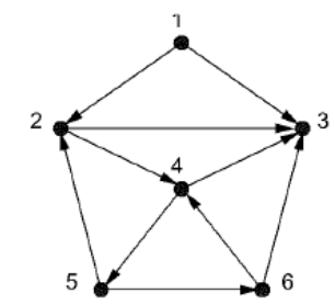 Figure 1
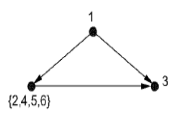 Figure 1
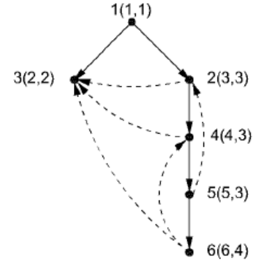 Figure 2
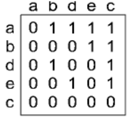 Figure 3
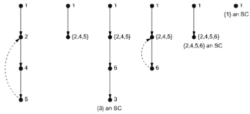 Figure 4
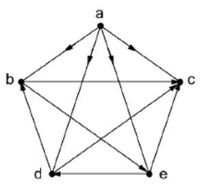 Figure 5
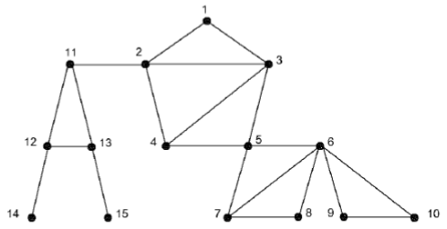 Figure 6
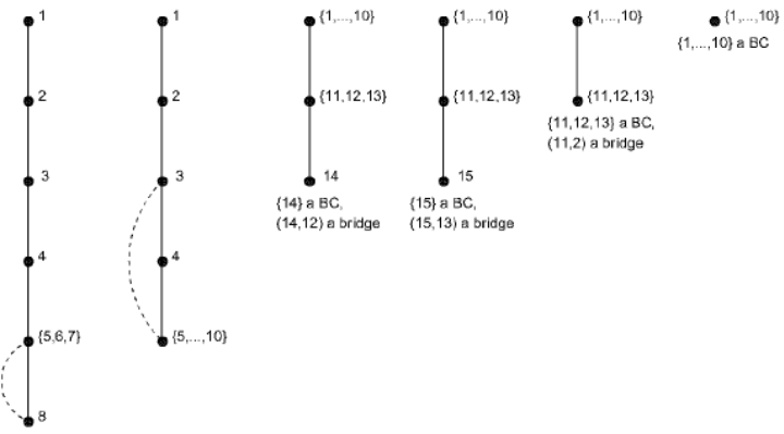 Figure 7
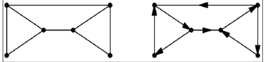 Figure 8
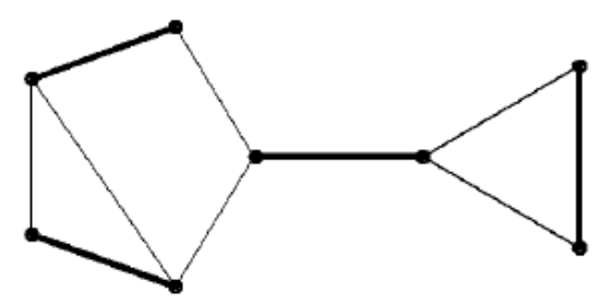 Figure 9
Introduction Strong Components of a Directed Graph
In this paper, G = (V, E) is a directed graph.
Definitions
For two vertices a and v, a uv-path is a path starting at a and ending at v. A directed graph G = (V, E) is strongly connected if for every two distinct vertices a and v, there is a uv-path and a vu-path. In general, a directed graph will not be strongly connected. But the vertices can be partitioned into blocks that are strongly connected, according to this definition: two vertices u v are in the same strong component (SC) if and only if they can reach each other, i.e., there is a uv-path and a vu-path. This defines a partition of V since it is an equivalence relation. For any directed graph G, contracting each SC to a vertex gives the strong component graph or condensation of G. A tournament is a directed graph G such that each pair of vertices is joined by exactly one edge. This models a round robin tournament, where edge (x, y) represents the inference that player x beat player y.
Inference
Let C be a cycle in a graph G. All vertices of C are in the same SC. Contracting the vertices of cycle C to a single vertex yields a graph with the same SC graph as G. The SC graph is always a Directed Acyclic Graph. A topological numbering of the SC graph of a tournament gives a ranking of the players.
To see why, note that if player x is in an SC with lower topological number than y, then the tournament contains the edge (x, y) not (y, x). Thus SC number I contains the players that are unequivocally in the top tier they all beat all other players. SC number 2 contains the 2nd tier players they all beat all other players except those in tier 1, etc. All the vertices on a cycle belong to the same SC. In inference the SC graph is formed by repeatedly contracting cycles, until no cycle remains. A sink s is a vertex of the SC graph. In inference the SC's are {s} and the SC's of G s. Each iteration grows P by starting with the previous P and extending it, if possible. The algorithm has a low-level implementation that finds the SC graph in linear time [11] . Sinks are deleted and Cycles are contracted using a stack to represent P and another stack to give the boundaries of contracted vertices in P. The algorithm discovers each SC as a sink of the SC graph. So the SC's can be numbered in topological order by the method of topological order Algorithm.
The first linear-time algorithm for strong components is due to Tarjan [1] . It computes a value called lowpoint(v) for each vertex v. lowpoint(v) is the lowest-numbered vertex (in preorder) in v's SC that is reachable from v by a path of (0 or more) tree edges followed by a back or cross edge (lowpoint(v) equals v if no smaller numbered vertex can be reached). The vertices with lowpoint(v) = v are the "roots" of the strong components. A third linear-time strong component algorithm is due to Sharir [3] and Kosaraju (unpublished; see also [4] ). It does a depth-first search, followed by a second depth-first search on the reverse graph. This makes good sense the first search discovers which vertices can reach which others, and the second search discovers which vertices can be reached by which others.
Examples
Figure 1 shows a directed graph, its three strong components, and its SC graph. Each strong component is strongly connected. An elementary misperception is that a strongly connected graph has a Hamiltonian cycle. The component {2, 4, 5, 6} illustrates that this is not always true.
Each vertex is labeled by its preorder number followed by its low point value. The given matrix M is interpreted as a directed graph, with mzj corresponding to edge (i, j). The adjacency matrix of Example1 is constructed, and the 1 for each edge (i, j) is replaced by the value m2j. The resulting block upper triangular matrix has less fill-in for Gaussian elimination and nice properties for other matrix operations [7] . Figure 4 below illustrates the execution of the algorithm on the graph.
Bridges and Cut points of an Undirected Graph
In this paper G = (V, E) is a connected undirected graph.
Examples
Figure 6 shows a graph with 3 bridges, 6 cut points, and 7 biconnected components. It illustrates that an end of a bridge is a cut point unless it has degree one. However, a cut point need not be the end of a bridge. If a communications network (e.g., Internet) has a bridge, that link's failure disables communication, i.e., there are sites that cannot send messages to each other. If the network has an articulation point, that site's failure also disables communication.
Inference
All vertices on a cycle are in the same BC. In inference the bridge tree is formed by repeatedly contracting cycles. A vertex x of degree < 1 is a vertex of the bridge tree. In inference the BC's are {x} and the BC's of G -x. The following is a high level algorithm for finding the bridges and bridge tree. It has a linear-time implementation almost identical to the strong component algorithm. We call the last vertex x of a dfs path a dead end if x has degree < 1.
Algorithm 3: Bridges Input: connected undirected graph G = (V, E) Output: bridge components and bridges of G repeat until G has no vertices: grow a dfs path P until a cycle is found or a dead end is reached cycle C: contract the vertices of C dead end x: mark {x} as a BC if x has degree 1, then mark its edge as a bridge of G A similar linear-time algorithm finds the cutpoints and biconnected components of an undirected graph [2] . The original linear-time dfs algorithm of Hopcroft and Tarjan for cutpoints and biconnected components [1] is based on the idea of lowpoints.
Start with a dfs tree T. Assume that the vertices are numbered in discovery order and that each vertex is identified with its discovery number. Define lowpoint(v) = min{v} U {w : some back edge goes from a descendant of v to w} Hopcroft and Tarjan proved that G is biconnected if and only if vertex 1 has exactly one child (which must be vertex 2); Figure 8 below illustrates Robbins's Theorem that a connected undirected graph has a strongly connected orientation if and only if it is bridgeless [5] . If one of the horizontal edges is deleted, making the other a bridge, then the graph has no strongly connected orientation. EX: Kotzig's Theorem states that a unique perfect matching must contain a bridge of G. Figure 9 shows a graph with a unique perfect matching matched edges are drawn heavy. Note that deleting the bridge of the matching gives another graph with a unique perfect matching. This idea can be used to efficiently find a unique perfect matching or show it does not exist. Whitney's Flipping Theorem asserts that a graph is planar if and only if each biconnected component is planar [6] .
Figures and tables from the paper
References
11 in the original paper- Tarjan RE. Depth-first search and linear graph algorithms, SIAM J. Comput. 1972; 1:146-160.
- Gabow HN. Path-based depth-first search for strong and biconnected components, Inf. Proc. Letters. 2000; 74:107-114.
- Sharir M. A strong-connectivity algorithm and its application in data flow analysis, Comp. and Math. With Applications. 1981; 7:67-72.
- Cormen TH, Leiserson CE, Rivest RL, Stein C. Introduction to Algorithms, Second Edition, McGrawHill, 2001.
- Robbins HE. A theorem on graphs, with an application to a problem in traffic control, Amer. Math. Monthly. 1939; 46:281-283.
- Whitney H. Non-separable and planar graphs, Trans. Amer. Math. Soc. 1932; 34:339-362.
- Harary F. Graph Theory, Addison-Wesley, Reading MA, 1969.
- Aho AV, Sethi R, Sharir M. A strong-connectivity algorithm and its application in data flow analysis, Comp. and Math. With Applications. 1981; 7:67-72.
- Alstrup S, Harel D, Lauridsen PW, Thorup M. Dominators in linear time. SIAM J. Comput. 1999; 28:2117-2132.
- Auslander L, Parter SV. On imbedding graphs in the plane, J. Math. and Mech. 1961; 10:517-523.
- Gabow HN. An ear decomposition approach to approximating the smallest 3-edge connected spanning subgraph of a multigraph, Proc. 13th Annual ACMSIAM Symp. on Disc. Algorithms, 2002, 84-93.