
Research article · 2017 · Full text
International Journal of Statistics and Applied MathematicsNegative binomial sum of random variables and modeling financial data
Volume 2(3) · Pages 44–51
Research areasFinancial Risk and Volatility ModelingComplex Systems and Time Series AnalysisFuzzy Systems and Optimization
Abstract
Author-writtenA limiting probability distribution of negative binomial sum of independently and identically distributed random variable is obtained, which we call Negative Binomial Stable (NBS) distribution. It is applied in the forecasting of market changes by fitting the pound exchange rate change in relation with the Indian rupees. Using the data we empirically compare normal, stable, geometric stable (GS) and NBS distributions. Among which the NBS distribution shows better fit than the normal, stable and GS models judged in terms of Kolmogrov distance test. The NBS model is a generalization of the GS model.
Summary
Source-checkedPlain-language reading of the full paper, prepared with AI and checked against the text. Each point links to the authors' own words.
Why it matters
- Early statistical modeling of stock price changes relied on the normal model, based on the central limit theorem's assumptions of independence, identical distribution, and finite variance. View evidence ↗
- Subsequent research found that stock returns exhibit higher kurtosis and heavy tails than the normal distribution, leading to the use of symmetric stable distributions. View evidence ↗
- Many alternative financial models are limited because they lack a basis in limiting probability distributions, do not have domains of attraction, and are not stable under scaling transformations. View evidence ↗
The question
- The authors aim to obtain and apply a limiting probability distribution for the negative binomial sum of i.i.d. random variables, termed the Negative Binomial Stable (NBS) distribution. View evidence ↗
What they did
- The NBS distribution is defined as a random variable stable with respect to a negative binomial summation scheme involving i.i.d. random variables and a negative binomial random variable T(r,p). View evidence ↗
- The authors use a version of the method of moments based on the sample characteristic function to derive explicit estimators for the distribution's parameters. View evidence ↗
- The model is tested using daily exchange rate changes of the British pound relative to the Indian rupee from January 1, 1990, to December 31, 1998. View evidence ↗
- The goodness of fit for the NBS distribution is compared against normal, stable, and geometric stable (GS) distributions using the Kolmogorov distance test. View evidence ↗
What they found
- The normal and stable distributions yielded Kolmogorov distances of 0.3590 and 0.3213, respectively, when fitted to the exchange rate data. View evidence ↗
- For the NBS distribution with r = 0.2, the Kolmogorov distance was 0.1195, indicating a closer fit than the normal or stable models. View evidence ↗
- When r = 1, the NBS distribution's Kolmogorov distance is 0.2377, which corresponds to the fit of the geometric stable (GS) distribution. View evidence ↗
- As the parameter r increases to 11, the Kolmogorov distance for the NBS distribution increases to 0.2999, showing a decrease in fit quality compared to lower r values. View evidence ↗
- The NBS distribution generally provides a better fit for the financial data than the normal, stable, and GS models based on the Kolmogorov distance test. View evidence ↗
What it means
- The authors conclude that the NBS model is superior to normal and stable models, and specifically outperforms the GS model when 0 < r < 1. View evidence ↗
- The authors note that while their estimation procedure works for all choices of t, the varying rate of convergence requires further investigation. View evidence ↗
Visual summary
2 visualsIllustrations explain the paper; charts are replotted from the paper's own table values.
NBS Summation Concept
AI-generated conceptual illustration (Abstract mathematical probability flow). It explains the idea and does not show study data.
View source evidence ↗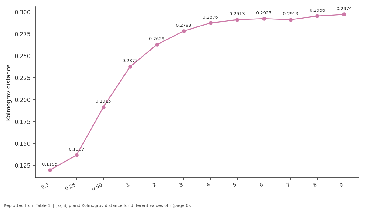
Kolmogrov distance: 0.2 vs 0.25 vs 0.50 vs 1 vs 2
Replotted from Table 1 (page 6) of the original paper. Every bar is the paper's own table value.
View source evidence ↗Figures & tables
From the original paper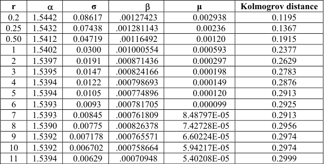 Table 1
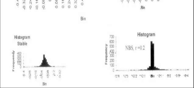 Figure 1
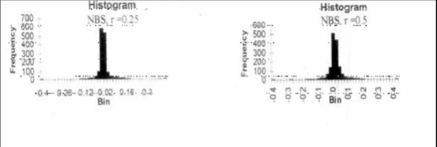 Figure 1
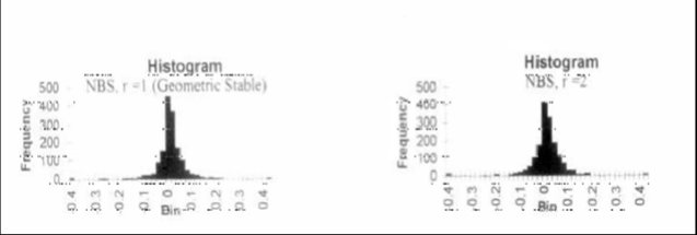 Figure 2
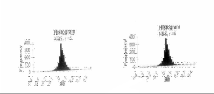 Figure 3
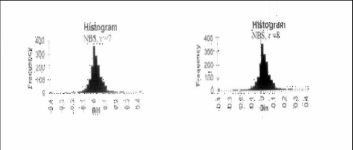 Figure 3
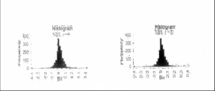 Figure 4
Introduction and Preliminaries
The probability distribution of negative binomial sum of independently and identically distributed (i.i.d) random variables is studied by many authors (Cooper 1998, Ergodan et al. 1998) [5,7] . Here we are presenting another application of a limiting probability distribution of negative binomial sum of i.i.d random variables, which has applications in economics, finance, management, mathematics, statistics, trade, commerce etc. The first step towards the statistical modeling of stock price changes was taken by Bachelier (1900) [2] . His idea reflects the realities of central limit theorem: (i) independence (ii) identical distribution and (iii) finite variance of daily changes. He used the normal model, since the price change over a period of time can be regarded as the sum of changes in shorter periods of time, weekly change = sum of daily changes, daily change = sum of changes between the various transactions. But further research in this area revealed the fact that the empirical distributions of stock returns had more kurtosis than the normal distribution (Mandelbrot 1963 a, b, and Fama 1965) [13, 14, 8] . They used symmetric stable distribution, since the family of stable distribution is the sum of i.i.d. random variables, have heavy tails and domains of attraction with respect to summation scheme. Thus the stable distributions are the only possible limits of (scaled) sum of i.i.d. random variables. This asymptotic property enables the researchers for using stable models to model this uncertainty. Since the normal model is a special case of stable distribution, it has got some popularity among financial modelers. But a number of empirical models (Officer 1972, Blattberg et al. 1974, Press 1982, Akgiray et al. 1988) [18,3,20,1] showed the inconsistency with the stable model. Because of this inconsistency DuMouchel (1973) [6] proposed a mixture of normal and stable model which has heavy tails. Boness et al. (1974) [4] proposed a mixture of normal distributions without heavy tails. Alternative contributions in this area of research is; Praetz (1972) [19] , Blattberg et al. (1974) [3] . But the main demerit of all these models is, they are not based on a limiting probability distribution and do not have domains of attraction and are not closed with respect to scaling under certain transformations, that is they are not stable. The scaling idea is contributed by Mandelbrot (1977) [12] . Mitlnik and Rachev (1989, 1991, 1993) [15][16][17] used the stability concept of Mandelbrot and proposed Weibull distribution, which arises in the geometric summation scheme and dominate all other alternative stable models. Distributions which arise from summation scheme can be classified by the single parameter, the index of stability determining the main properties of the distribution.
Kozubowski and Rachev (1994) [10] proposed GS model and have shown that the GS model successfully compete with the normal and stable model by fitting Yen exchange rate changes (in relation to the US dollar). Where Yen is the unit of Japanese currency. The NBS model considered in this paper belongs to the stable family, has domains of attraction and heavy tails. The model successfully competes with the normal and stable model. It also better fit the pound exchange rate change than the GS model for some specific values of the parameters. The GS model is a particular case of the NBS model. Here is the organization of the paper: section 2 deals with preliminary definitions and properties, section 3 presents representations and simulations. Section 4 deals with application for modeling financial data. Section 5 deals with numerical simulation results and section 6 is for conclusion.
Preliminary Definitions and Properties
A random variable (r.v.) Y with distribution function G is said to be stable with respect to negative binominal summation scheme, if there exists a sequence of i.i.d random variables X1, X2, …, a negative binomial random variable T(r,p) independent of all Xi, and constants a(p) > 0 and b(p) Є R such that
Since T (r, p) converges in distribution to the gamma distribution with parameter r as p→ 0, Y has the characteristic function Ψ (t) =λ (-logф (t)), Where λ is the Laplace transform of the gamma distribution with parameter r and ф(t) is the characteristic function of an α-stable distribution.
We call the limiting distribution Y, as NBSα(σ, β, μ, r). The parameters: α (0 < α ≤ 2) is the characteristic exponent or the index of stability, determines the main characteristics of the distribution,σ (σ > 0) is the scale parameter, β ( |β| ≤ ) is the intensity of skewness and μ (μ R) is the shift parameter. Proof follows from Kozubowski et al. (1996) [9] Example The gamma distribution with ch.fn. Ψ (t) = (1-iμt) -r belongs to the NBS family of distributions. The corresponding stable distribution is the degenerate distribution with ch.fn. exp(itμ).
Property 2.1
NBS distribution is closed under finite convolution for same , σ, β, μ:
Yr is asymptotically -stable as r .
Estimation of Parameters: Moment Estimation
An analytical procedure which yields explicit estimators and involves minimal computation is a version of method of moments based on sample characteristic function.Let Y1, Y2, ………,Yn be i i.d. copies of Y with characteristic function Ψ represented by (2.1)-(2.3). The function
By strong law of large numbers (SLLN) ψ n(t) Ψ(t) (a.s ) as n An analytic procedure which yields explicit estimator for the parameter 'r 'is difficult and sometimes impossible. We estimate the parameters α, σ, β and µ for different values of the parameter 'r' Let U(t) and V(t) be the real and imaginary parts of Ψ(t) (-1/r) -1 respectively. For any t i > 0 (t i ≠ t j ), ( i,j =1,2,3,...)
gives the estimators α and λ of and respectively.
2) Choose two non-zero values of t; say t 3 and t 4 such that t 3 t 4. Then for = 1
Case of = 1
Letting V(t) be the imaginary part of Ψ(t) (-1/r) -1. , the estimators are consistent. The procedure holds good for all choices of t (- < t < ), but the rate of convergence may be different. This requires further study.
Representation and Simulation
The most widely used technique of simulation of random variables is the well-known inversion method (Devroye 1986). If a random variable X has the distribution funtion F, then (U) F X 1 d , where F -1 is the inverse of F and U is a uniform random variable on (0, 1). Since generally there are no analytic expressions for the NBS distribution functions and their inverses, the inversion method is not applicable to the NBS case. The computer simulation algorithm for the NBS distribution has the following steps.
A general NBS () generator (i) Generate a standard gamma variate Z with parameter r. (ii) Generate a standard stable variate X ~ S (1, , 0) independent of Z.
(iv) RETURN Y Simulating a standard stable X ~ S (1, , 0) random variable consists of the following steps. 1. Generate a standard exponential variate W.
Generate uniform
Following we provide a representation of the random variable Y in terms of a gamma random variable with parameter r and stable random variable.
where X ~ S(1, β, 0) and Z is standard gamma independent of X. Proof follows from Kozubowski and Panorska (1996) [9] Proposition 4.2 Let X ~ S ( σ, 0, 0) with 0 < 2 and let 0 < < . Let Y be NBS/ random variable totally skewed to the right.
Then W d X Y 1/ ~ NBS (σ, 0, 0) Proof Let x (t) and w(t) be the ch.fn of X and W respectively.
where Z is standard gamma and U ~ S/((cos(/2)) / 1, 0) and U has the Laplace transform E exp (-U) =exp (-
The right side is the ch.fn. of NBS (σ,0,0) Which completes the proof.
Applications to Modeling Stocks
Here we are presenting the NBS distribution to model the pound exchange rate change in relation to Indian rupees. It is assumed that the exchange rate change in one day is the sum of a large number of changes occurred in that day. The number of changes may not be deterministic. It may be random. While using the normal and stable distributions to model the financial data, the number of changes in one day is deterministic. But it is not a realistic assumption. There may be an independent number of random innovations. Hence it is a r.v.. Kozubowski and Rechav (1994) [10] proposed the GS distribution for modeling financial data sets, where it is assumed that the number of changes in one day follows the geometric distribution and the parameter p stands for the probability of a dramatic change in the market during each period. But in our model we are assuming that the number of changes in one day follows the negative binomial distribution. Thus if Y represents the change of a commodity in one day, thus change in one day = ρ) T(r, 1 i "small changes". In terms of random variables, the daily price change Y = X1+X2+ …… + XT(r,), where Xi represents price change between successive transactions and are assumed to be independently and identically distributed random variables. The negative binomial random variable T(r,p) represents the time at which the probabilistic structure governing the returns break down. p denotes the probability of small changes and r is time required for that change. We can observe that the price value of the shares of certain companies changes very rapidly and even we cannot record that change. These changes are occurred even within a small fraction of a second. From the table 1 we can conclude that the NBS distribution better fits those data sets where the price value changes very rapidly.
| r | | σ | | μ | Kolmogrov distance |
|---|---|---|---|---|---|
| 0.2 | 1.5442 | 0.08617 | .00127423 | 0.002938 | 0.1195 |
| 0.25 | 1.5432 | 0.07438 | .001281143 | 0.00236 | 0.1367 |
| 0.50 | 1.5412 | 0.04719 | .00116492 | 0.00120 | 0.1915 |
| 1 | 1.5402 | 0.0300 | .001000554 | 0.000593 | 0.2377 |
| 2 | 1.5397 | 0.0191 | .000871436 | 0.000297 | 0.2629 |
| 3 | 1.5395 | 0.0147 | .000824166 | 0.000198 | 0.2783 |
| 4 | 1.5394 | 0.0122 | .000798693 | 0.000149 | 0.2876 |
| 5 | 1.5394 | 0.0105 | .000774896 | 0.000120 | 0.2913 |
| 6 | 1.5393 | 0.0093 | .000781705 | 0.000099 | 0.2925 |
| 7 | 1.5393 | 0.00845 | .000761809 | 8.48797E-05 | 0.2913 |
| 8 | 1.5390 | 0.00775 | .000826378 | 7.42728E-05 | 0.2956 |
| 9 | 1.5392 | 0.007178 | .000765571 | 6.60224E-05 | 0.2974 |
| 10 | 1.5392 | 0.006702 | .000758664 | 5.94217E-05 | 0.2974 |
| 11 | 1.5394 | 0.00629 | .00070948 | 5.40208E-05 | 0.2999 |
Table text extracted from the original PDF; superscript letters are shown inline. The original table image is below.
View original table image
Numerical Simulation
We shall consider the distribution of pound exchange rate changes in relation with the Indian rupees, where pound is a unit of Britan currency. The data are daily exchange rate changes from 1-1-1990 to 31-12-1998. The data is fitted for normal, stable, geometric stable and NBS distributions. As usual we consider the change in the log (price) from t to t + 1 that is each data point Pt = 1n (Xt+1) -ln(Xt), where Xt represents the closing price of the commodity on day t. As shown in the histogram of data, the peaked ness is the characteristic of many financial data sets. We use maximum likelihood estimators for estimating μ and σ for the normal distribution. The parameters in stable and GS distributions are estimated by the method of moments (Kozubowski 1998, Press 1972) [21] . The technique explained in section (3) is followed for estimating parameters of NBS distribution. Observations are simulated from respective distributions and histograms are drawn for the data set and the simulated values (fig 1234). Because of the scaling, the small frequencies are not visible in the histogram. Kolmogrov distance test is conducted to test the goodness of fit of the distributions.
For the normal distribution μ ˆ=0.00061943 and σ ˆ=0.06395, for stable distribution α ˆ=1.5392, σ ˆ=0.0299, β ˆ=0.0469 and μ =0.000594.
For the normal and stable distributions the Kolmogrov distance is 0.3590 and 0.3213 respectively.The table 5.1 shows the estimated values of , σ and μ for different values of r, of NBS distribution. The table also shows the Kolmogrov distance for simulated observations. When r = 1, we get the estimators and Kolmogrov distance of the geometric stable distribution.
Conclusions
The Kolmogrove distance test shows that the NBS distribution better fit the pound exchange rate change than the normal and the stable model. For r = 1, we get the goodness of fit of the geometric stable distribution. For 0 < r < 1, the NBS model successfully compete with the normal, stable and GS models.
Figures and tables from the paper
References
21 in the original paper- Akgiray V, Booth GG. The stable law model of stock returns, Journal of Business and Economics Statistics. 1988, 51-57.
- Bachelier L. Theorie de law speculation, Annals de I'Ecole Normale supericure series. 1900; 3:21-86.
- Blattberg RC, Gonedes NJ. A comparison of stable and Student distribution as statistical methods for stock prices, Journal Business. 1974; 47:224-280.
- Boness A, Chen AJ, Atusipitak S. Investigation of non-stationary prices, Journal of Business. 1974; 47:518-537.
- Cooper W. Negative binomial sums of random variables and discounted reward processes, J. Appl. Prob. 1998; 35:589-599.
- Du Mouchel W, Stable distributions in statistical inference: Symmetric stable distribution compared to other symmetric longtailed distributions, Journal of American Statistical Association. 1973; 68:469-477.
- Ergodan B, Ostrovskii. Analytic and asymptotic properties of generalized. Linnik probability density, J. Math. Anal. Appl. 1998; 227:555-578.
- Fama E. The behaviour of stock market prices prices, Journal of Business. 1965; 38:34-105.
- Kozubowski TJ, Panorska AK. On moments and tail behaviour of v-stable random variables, Statistics and Probability letters. 1996; 29:307-315.
- Kozubowski TJ, Rachev ST. The theory of geometric stable distributions and its use in modeling financial data, European Journal of Operational Research. 1994; 74:310-324.
- Kozubwski TJ. Estimation of parameters of stable laws, J Math. Comput. Modelling, 1998.
- Mandelbrot B. The Fractal Geometry of Nature, Freeman, New York, 1977.
- Mandelbrot B. New methods in statistical economics, Journal of Political Economy. 1963; 71:421-440.
- Mandelbrot B. The variation of certain speculative prices, Journal of business. 1963; 26:394-419.
- Mittnik S, Rachev ST. Stable distributions for asset returns, Applied Mathematics Letters. 1989; 2:301-304.
- Mittnik S, Rachev ST. Alternative multivariate stable distributions their applications to financial modeling. 1991, 107-119.
- Mittnik S, Rachev ST. Modeling asset returns with alternative stable distributions, Economic Review. 1993; 12:261-330.
- Officer RR. The distribution of stock returns, Journal American Statistical Association. 1972; 76:807-812.
- Praetz P. The Distribution of share price changes, Journal of Business. 1972; 47:49-55.
- Press SJ. Applied Multivariate Analysis, 2 nd ed., Krieger, Malabar, 1982.
- Press SJ. Estimation in univariate and multivariate stable distributions, Journal of the American Statistical Association. 1972; 67:842-846.
Cited by 6
From OpenAlex, OpenCitations and reference lists read by Scinovex
- Bounds for convergence rate in laws of large numbers for mixed Poisson random sums ↗
Victor Yu. Korolev, Alexander I. Zeifman · Statistics & Probability Letters · 2020
❝ 10PDF - On the Order of Approximation in Limit Theorems for Negative–Binomial Sums of Strictly Stationary m-Dependent Random Variables ↗
Trần Lộc Hùng, Phan Tri Kien · Acta Mathematica Vietnamica · 2021
❝ 1 - An Extension of Zolotarev’s Problem and Some Related Results ↗
Trần Lộc Hùng, Phan Tri Kien · Acta Mathematica Scientia · 2021
❝ 1 - Asymptotic behaviors with convergence rates of distributions of negative-binomial sums ↗
Trần Lộc Hùng, Phan Tri Kien, Nguyen Tan Nhut · Science and Technology Development Journal · 2020
The negative-binomial sum is an extension of a geometric sum. It has been arisen from the necessity to resolve practical problems in telecommunications, network analysis, stochastic finance and insurance mathematics, etc. Up to the present, the topics related to negative-binomial sums like asymptotic distributions and rates of convergence have been investigated by many mathematicians. However, in a lot of various…
❝ 1PDF - Convergence in Total Variation of Random Sums ↗
Luca Pratelli, Pietro Rigo · Mathematics · 2021
Let (Xn) be a sequence of real random variables, (Tn) a sequence of random indices, and (τn) a sequence of constants such that τn→∞. The asymptotic behavior of Ln=(1/τn)∑i=1TnXi, as n→∞, is investigated when (Xn) is exchangeable and independent of (Tn). We give conditions for Mn=τn(Ln−L)⟶M in distribution, where L and M are suitable random variables. Moreover, when (Xn) is…
❝ 0PDF - On the Rate of Convergence in Limit Theorems for Negative–Binomial Random Sums ↗
Trần Lộc Hùng, Phan Tri Kien · Lobachevskii Journal of Mathematics · 2021
Abstract The main purpose of this paper is to study the rate of convergence in limit theorems for normalized negative–binomial random sums of independent, identically distributed random variables. The obtained limit distributions correspond to a so-called class of Negative–Binomial Infinitely Divisible distributions. Zolotarev’s probability metric is used as a main research approach in this paper.
❝ 0