
Research article · 2017 · Full text
International Journal of Statistics and Applied MathematicsAnalytical expressions of a steady MHD viscous incompressible fluid flow through a porous planner channel
Volume 2(2) · Pages 12–17
Research areasNanofluid Flow and Heat TransferFluid Dynamics and Turbulent FlowsHeat and Mass Transfer in Porous Media
Abstract
Author-writtenIn this paper we investigate the oscillatory flow of a steady MHD viscous incompressible fluid with radiative heat transfer analysis through a porous planar channel filled with a saturated porous medium in slip condition is considered. It is guessing that the no-slip condition between the wall and the fluid remains no longer valid. The approximate analytical expressions the dimensionless axial velocity, dimensionless temperature and the slip parameters for the non-linear boundary value problem are derived. We also discuss the graphical representations of the dimensionless velocities, dimensionless temperatures are also discussed.
Summary
Source-checkedPlain-language reading of the full paper, prepared with AI and checked against the text. Each point links to the authors' own words.
Why it matters
- Viscous flow analysis is critical for various engineering applications, including heat transfer problems and the study of turbulent boundary layers. View evidence ↗
- Magnetohydrodynamics (MHD) fluid flow, which involves magnetic fields and heat transfer, is utilized in nuclear reactors, plasma studies, and geothermal energy extraction. View evidence ↗
- While the no-slip condition is common, Navier proposed a slip boundary condition where fluid velocity at a surface is proportional to the shear stress. View evidence ↗
The question
- The study aims to investigate the oscillatory flow of a steady MHD viscous incompressible fluid with radiative heat transfer through a porous planar channel under slip conditions. View evidence ↗
What they did
- The researchers modeled an incompressible, electrically conducting fluid within a saturated porous medium channel, subjected to a homogeneous magnetic field and radiative heat transfer. View evidence ↗
- The non-linear differential equations governing the flow were solved using the Homotopy Analysis Method (HAM). View evidence ↗
- An auxiliary parameter, h, was utilized within the HAM to control the convergence rate and region of the series solution. View evidence ↗
What they found
- An increase in the radiation parameter (N) leads to an increase in the dimensionless temperature profile, assuming other parameters remain fixed. View evidence ↗
- The axial velocity profile increases as the Grashoff number (Gr) increases, given fixed values for other parameters. View evidence ↗
- An increase in the Hartmann number (H) results in a decrease in the axial velocity profile. View evidence ↗
- The axial velocity profile decreases when the porous medium shape factor (S) increases. View evidence ↗
- The axial velocity profile increases as the radiation parameter (N) increases. View evidence ↗
- An increase in the slip parameter (γ) leads to an increase in the axial velocity profile. View evidence ↗
Figures & tables
From the original paper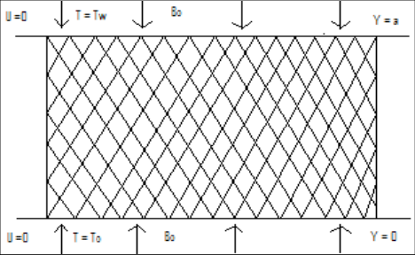 Figure 1
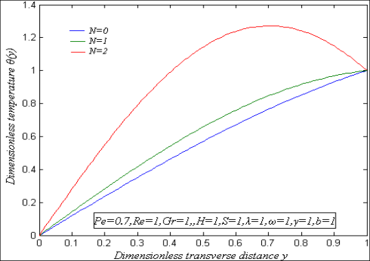 Figure 2A
 Figure 2B
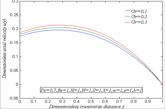 Figure 3
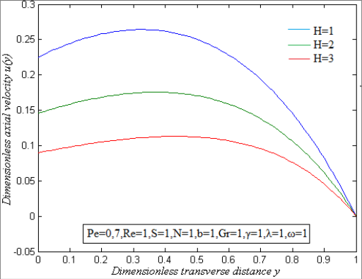 Figure 3
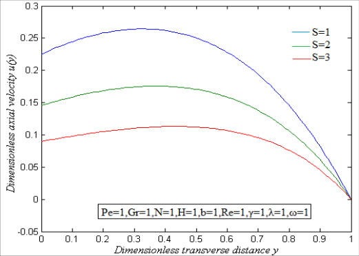 Figure 3
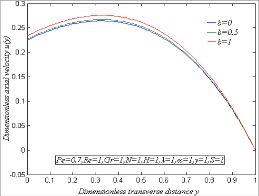 Figure 3
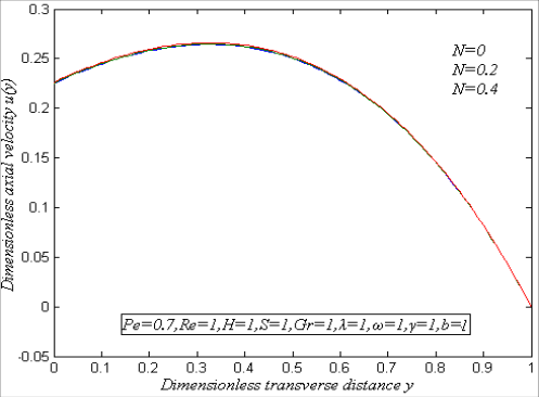 Figure 3
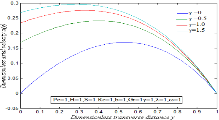 Figure 3
Introduction
Viscosity can be defined through the relation between the shear stress, and force per unit area F/A, needed to keep the upper plate moving with a constant velocity [1] . Applications of viscous flow are turbulent boundary layer, flat plate frictional law, application to heat transfer problems (boundary layer energy equations, similar solution for energy equation in flat plate, integral method, convective thickness, velocity and temperature distributions, Stanton number, Couette flow assumption and numerical solution of differential equations).When a viscous fluid flows over a solid surface, there is no relative motion between the fluid and the solid at the interface. Under normal circumstances, the no-slip condition provides a realistic restriction on solutions of the Navier-stokes equation ( [2] ). The boundary condition for a viscous fluid at a solid wall is one of no-slip, i.e. the fluid velocity matches the velocity of the solid boundary. Navier proposed a general boundary condition that incorporates the possibility of fluid slip at a solid boundary. Navier's proposed condition assumes that the velocity, x V at a solid surface is proportional to the shear stress at the surface (Navier [3] , Goldstein [4] ).
Where, is the slip strength or slip coefficient. If =0 then the general assumed no-slip boundary condition is obtained. If is finite, fluid slip occurs at the wall but its effect depends upon the length scale of the flow. A fluid in direct contact with a solid sticks to the surface due to viscous effects, and there is no slip. The flow region adjacent to the wall in which the viscous effects (and thus the velocity gradients) are significant is known as boundary layer. Viscous flow region-flows in which the frictional effect is significant [5] . Fluid flow under the influence of magnetic field and heat transfer occurs in magneto-hydrodynamics accelerators, pumps and generators. This type of fluid has uses in nuclear reactors, plasma studies, geothermal energy extraction, and the boundary layer control in the field of aerodynamics [6] . By applying the perturbation technique Kumar et al. [8] investigated the same problem of slipflow regime for the unsteady MHD periodic flow of viscous fluid through a planer channel. Hayat et al. [7] studied heat transfer and slip flow of a second grade fluid past a stretching sheet through a porous space.
Mathematical formulation of the problem
Assume that the flow of an incompressible viscous and electrically conducting fluid in a channel filled with saturated porous medium under the influence of an externally applied homogeneous magnetic field and radiative heat transfer as shown in Fig. 1.
Fig 1: Geometry of the problem
It is assumed that the fluid has small electrical conductivity and the electromagnetic force produced is very small. Take a Cartesian coordinate system ,where,x o lies along the centre of the channel, y is the distance measured in the normal section. Then, assuming Boussinesq incompressible fluid model, the equations governing the motion are given by
The corresponding boundary conditions are as follows:
It is assumed that both walls temperature w T T , 0 are high enough to induce radiative heat transfer. It is also assumed that the fluid is optically thin with a relatively low density and the radiative heat flux is given by
Where is the mean radiation absorption coefficient. We introduce the dimensionless variables and parameters are as follows:
Where U is the flow mean velocity, the dimensionless governing equations together with the appropriate boundaries conditions, can be written as
The steady flow eqns. of ( 7) and ( 8) are as follows:
The corresponding boundary conditions are as follows:
Where Gr means Grashoff number, H indicates Hartmann number, N denotes Radiation parameter, Pe represents Peclet number,Re refers Reynolds number, Da means Darcy number and S denotes porous medium shape factor parameter.
Solution of the non-linear boundary value problem
In recent days, a basic tool for solving non-linear problem in Homotopy analysis method (HAM) which was generated by Liao [12] , is employed to solve the non-linear differential equation. The Homotopy analysis method is based on a basic concept in topology, i.e. Homotopy by Hilton [13] which is widely applied in numerical techniques as in [14][15][16] . Homotopy analysis method is independent of the small/large parameters not like the perturbation techniques [17] . There is a simple way to adjust and control the convergence region and rate of approximation series in Homoyopy analysis method. The Homotopy analysis method has applied in many non-linear problems such as heat transfer, viscous, non-linear oscillations [18] , non-linear water waves [22] , etc. Such varied successful applications of the Homotopy analysis method to conform its validity for non-linear problems in science and engineering. The auxillary parameter h is used to adjust and control the convergence of the series solution. In [27] , mathematical expression is solved using the Homotopy analysis method. In this paper, the non-linear boundary value problem which is expressed in the eqns. ( 9) -( 12) can be solved directly. The approximate analytical expressions for the dimensionless axial velocity y u and dimensionless temperature y are as follows:
Figures and tables from the paper
References
23 in the original paper- Newmann J. Physics of the life sciences, Springer science and Business Media, LLC. 2008.
- Navier CLMH, Mem Acad. Sci. Inst. France. 1823; 1:414-416.
- Goldstein S. Modern Developments in Fluid dynamics, Dover, New York. 1995; 2:676.
- Hayat T, Javed T, Abbas Z. Slip flow and heat transfer of a second grade fluid part a stretching sheet through a porous space. Int. J of Heat and Mass transfer. 2008; 51:4528-4534.
- Kumar A, Arshney CLV, LAL S, MHD. Coquette flow with heat transfer and slip flow effects in an inclined channel, Journal of Mathematics. 2001; 43:47-62.
- Makinde OD. Magneto-hydrodynamic stability of planePoiseuille flow using multideck asymptotic technique, Mathematical and Computer Modelling. 2003; 37(34):251-259.
- Makinde OD, Sibanda P. Wall driven steady flow and heat transfer in a porous tube, Comp. Assist. Mech. Eng. Sc. 1998; 5:389-398.
- Jha BK, Ajibade AO. Free convective flow between vertical porous plates with periodic heat input, ZAMM Z. Angew. Math. Mech. 2010.
- Liao SJ. The proposed Homotopy analysis technique for the solution of nonlinear problems, PhD thesis, Shanghai JiaoTong University. 1992.
- Hilton PJ. An introduction to Homotopy theory, Cambridge University Press. 1953.
- Alexander JC, Yorke JA. The Homotopy continuation method: numerically implementable topological procedures. Trans. Am. Math. Soc. 1978; 242:271-284.
- Chan TFC, Keller HB. Arc-length continuation and multi-grid techniques for non-linear elliptic eigenvalue problems, 173-193. SIAM J. Sci. Statist. Comput., 3, 1982.
- Dinar N, Keller HB. Computations of taylor vortex flows using multigrid continuation methods, Tech. Rep. California Institute of Technology. 1985.
- Cole JD. Perturbation Methods in Applied Mathematics, Blaisdell, 1958.
- Liao SJ, Campo A. Analytic solutions of the temperature distribution in Blasius viscous flow problems. J Fluid Mech. 2002; 453:411-425.
- Liao SJ. An explicit, totally analytic approximation of Blasius viscous flow problems. Intl J. Non-Linear Mech. 1999; 34:759-778.
- Yu S, Amed TA. Slip-flow heat transfer in rectangular microchannels, Int. J Heat Mass Transfer. 2002; 44:42254234.
- Watanebe K, Yanuar H. Mizunuma. Slip of Newtonian fluids at solid boundary, JSME Int. J Ser., B41, 525, 1998.
- Liao SJ, Cheung KF. Homotopy analysis of non-linear progressive waves in deep water, J Engg. Maths. 2003, 45.
- Ruckenstien E, Rajora P. On the no-slip boundary conditions of hydrodynamics, J Collied Interface Sci., 1983; 96:488-491.
- Asghar S, Hanif K, Hayat T. The effect of the slip condition on unsteady flow due to non-coaxial rotations of disk and a fluid at an infinity, Meccanica. 2007; 42:141-148.
- Makinde OD, Osalusi E. MHD steady flow in a channel with slip at the permeable boundaries, Rom. J. Phys. 2006; 51:319-328.
- Ananthaswamy V, Soumyadevi J. Mathematical expressions of heat transfer to MHD oscillatory flow and Homotopy analysis method, International Journal of Mathematics and its Applications. 2016; 4(1-D):175-187.