
Research article · 2017 · Full text
International Journal of Statistics and Applied MathematicsA unified formula of a series of exact solutions for coupled Schrödinger-KdV equation
Volume 2(1) · Pages 25–30
Research areasNonlinear Waves and SolitonsFractional Differential Equations SolutionsNonlinear Photonic Systems
Abstract
Author-writtenIn this paper, a unified formula of a series of exact solutions for the coupled Schrodinger-KdV equation is obtained by using Hirota bilinear method and trial function method. These solutions contain bi-soliton solution, singular periodic amplitude solution and breather soliton solution. The results contribute to a better understanding of the structure of the solutions and non-linear phenomena for the coupled Schrodinger-KdV equation.
Summary
Source-checkedPlain-language reading of the full paper, prepared with AI and checked against the text. Each point links to the authors' own words.
Why it matters
- The coupled Schrödinger-KdV equation is used to model the nonlinear interaction between long and short waves. View evidence ↗
- Depending on the control parameters, the system can exhibit chaotic motion or recurrence. View evidence ↗
The question
- The authors aim to find a unified formula for exact solutions of the coupled Schrödinger-KdV equation, specifically targeting breather soliton solutions which they state have not been previously reported. View evidence ↗
What they did
- The research employs the Hirota bilinear method and the trial function method to derive the solutions. View evidence ↗
What they found
- The authors successfully derived a unified solution set that encompasses soliton, periodic amplitude, and breather soliton solutions. View evidence ↗
What it means
- The authors conclude that their findings increase the known diversity of wave structures for the coupled Schrödinger-KdV equation. View evidence ↗
Visual summary
1 visualsIllustrations explain the paper; they do not show study data.
Unified Solution Framework
AI-generated conceptual illustration (Mathematical wave functions in a quantum-fluid system). It explains the idea and does not show study data.
View source evidence ↗Figures & tables
From the original paper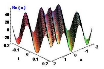 Figure 1
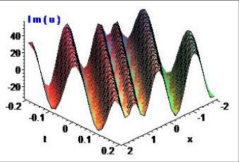 Figure 1
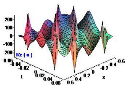 Figure 2
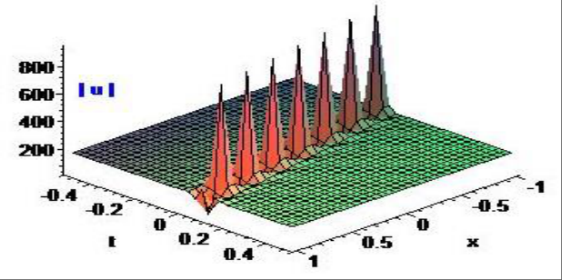 Figure 3
Introduction
Takao Yoshinaga et al. studied nonlinear interaction between long and short waves from the following model, which was called coupled Schrödinger-KdV equation [1]. iu u uv t xx 2 , v vv v u ( ) , t x xxx x (1) where ( , ) u u x t and ( , ) v v x t denote, respectively, the complex amplitude of the short wave and the long wave, and x and t are the normalized space-time coordinates, while and are control parameters. The positive or negative sign in front of xx u should be adopted depending upon the property of the medium. Their study results exhibit recurrence or chaotic motion, depending upon the magnitude of the control parameters involved in the governing equations (1). Many researchers have investigated the special case of Eqs.(1), that is the following form [2-5]. iu u uv t xx 2 , v vv v u 6 ( ) . t x xxx x Maths 2017; 2(1): 25-30 Changfu Liu School of Mathematics, Wenshan University, Wenshan, China Jinmei Liu School of Mathematics, Wenshan University, Wenshan, China Ping Zhou School of Mathematics, Wenshan University, Wenshan, China Min Chen School of Mathematics, Wenshan University, Wenshan, China Correspondence Changfu Liu School of Mathematics, Wenshan University, Wenshan, China (2) Such as Dogan Kaya and Salah M.
El-Sayed obtained the exact and approximate traveling- wave solutions for Eqs.(2) by using the Adomian's Decomposition Method [2]. Ardeshir Ahmadi Siahdareh and his colleagues found analytical solutions of Eqs.(2) through a hybrid of Fourier Transform and Adomian Decomposition Method [3]. A number of Jacobi-elliptic function solutions, soliton-like solutions and trigonometric-function solutions were also obtained by A. Filiz et al. by using F-expansion Method [4].
While numerical analysis of Eqs.(2) is studied by S. Kücükarslan through the Homotopy Perturbation Method [5]. To our knowledge, breather soliton solutions of Eqs.(2) have not been reported. The aim of the present paper will be to investigate Eqs.(2) by using Hirota bilinear method and trial function method, and to obtain a unified formula of a series of exact solutions including soliton solution, periodic amplitude solution and breather soliton solution [6, 7]. 2 Exact solutions to Schrödinger-KdV equation First, we find 2 ( ( )) 2 0 0 ( , ) ( ) , ( , ) i kx at u x t a k e v x t a k (3) is a solution of Eqs.(2).
Second, we set xx G x t u x t v x t v F F x t 0 ( , ) ( , ) , ( , ) 2(ln ) , ( , ) (4) where 2 0v a k , then Eqs.(2) can be changed into the following bilinear equations with respect to F and G 2 iD D v G F ( ) 0, t x 0 ( 6 ) 0, D D D v D C F F G t x x x 2 4 2 0 (5) where C is a integration constant. In the calculation, Eqs.(5) is written as another form i FG FG FG F G F G v GF ( ) ( 2 ) 0, t t xx x x xx 0 2( ) 2( 4 3 ) 12 ( ) 0, FF F F FF F F F v FF F CF GG xt x t xxx xxxx x xx xx x 2 2 2 * 0 (6) where the asterisk denotes complex conjugate. Now, assuming that Px Qt Px Qt , , 1 2 3 i kx at Px Qt Px Qt F x t a e a e a cos Kx Lt G x t v e b e b e b cos Kx Lt b sin Kx Lt , , 0 1 2 3 4 (7) where ( 1,2,3), ( 1,2,3,4) i j a i b j , , , P Q K and L are constants to be determined, we substitute Eqs.(7) into Eqs.(6), some equations with respect to ( 1,2,3), ia i ( 1,2,3,4) jb j , , , P Q K and L can be obtained (the tedious calculation process is omitted). Solving these equations, we obtain the following results a a k k a a a a a k k a a a b b a k a a a a k a a a (3 3 )(4 ) (3 3 )(4 ) 2 2 , , 2 ( )(4 ) 2 ( )(4 ) 2 2 2 2 1 1 2 3 2 1 2 3 1 2 2 2 2 2 1 2 3 1 2 3 a a k k a a a a a a a k k b b C a k a a a a a a (3 3 )(4 ) (4 )(3 3 ) 2 1 , 0, , 2 ( )(4 ) 2 4 2 2 2 2 2 3 1 2 3 1 2 3 3 4 2 2 2 1 2 3 1 2 3 2 2 2 a k k P 3 3 4 a a a a k k a k k Q k a K a a a a a a a a (3 3 ) 3 3 , 2 , 2 , 4 4 1 2 3 3 2 2 2 1 2 3 1 2 3 1 2 3 2 1 2 a a a k k L k (3 3 ) 4 4 a a a 2 1 2 3 (8) where 1 2 3 , , , a a a a and k are arbitrary constants.
Then, we have 2 2 a k k a k k a x kt a x kt a a a a a a 3 3 2 2 1 2 3 1 2 3 3 3 3 3 2 ( 2 ) ( 2 ) 4 4 1 2 F( , ) = e e cos(2 ), x t a a a 2 3 a a a k k x kt a a a (3 3 ) ( 2 ) 4 2 1 2 3 1 2 2 3 ( 2 ) 4 k k a x kt a a a a k k a a x kt a a a i kx at 3 2 1 2 3 3 2 1 2 3 3 3 3 2 2 ( 2 ) 4 ( ) 1 2 3 G x t ( , ) e e 4 (4 )(3 3 ) 2 2 a a a a k k e a a a a a 1 2 2 1 2 3 a a a k k a x kt a a a (3 3 ) ( cos( 2 )) 2 , 4 2 1 2 3 2 1 2 3 (9) Substituting Eqs.(9) into Eqs.(4), we can obtain solutions of Schrödinger-KdV equation(2) as follows u x t ( , ) 2 2 a k k a k k a x kt a x kt a a a a a a i kx at 3 3 2 2 1 2 3 1 2 3 3 3 3 3 2 2 ( 2 ) ( 2 ) 4 4 ( ) 1 2 3 a a e e 1 2 (4 )(3 3 ) 2 ( 2 4 a a a a k k e a a a 2 1 2 3 2 1 2 a cos(2 )) 3 a a a k k x kt a (3 3 ) ( 2 ) 4 a a 2 1 2 3 2 2 ( 2 ) 3 3 3 3 ( 2 ) 4 4 a k k a k k a x kt a a a a a x kt a a 3 2 1 2 3 3 2 1 2 3 ( e e a a 1 2 2 1 2 a cos(2 )), 3 a a a k k x kt a a a (3 3 ) ( 2 ) 4 2 1 2 3 a k k a x kt a a a a k k a x kt a a a 2 2 2 3 3 ( 2 ) 3 2 3 2 4 1 2 3 1 2 3 3 3 2 ( 2 ) 4 3 v x t a k ( , ) e 2 (3 3 ) ( 4 a a k k a a e a a a a a 1 3 2 3 2 1 2 3 2 1 2 4 cos(2 ) a ) a a a k k x kt a a a a (3 3 ) ( 2 ) 4 1 2 2 1 2 3 2 2 3 3 3 3 ( 2 ) ( 2 ) 4 4 a k k a k k a x kt a x kt a a a a a a 3 3 2 2 1 2 3 1 2 3 ( e e a a 1 2 2 a k k a x kt a a a 2 3 2 1 2 3 3 3 2 2 ( 2 ) 4 1 2 a a a cos(2 )) 2 ( ) e (3 3 ) 3 3 ( 2 3 3 1 a a a k k a k k x kt a a a a a a ( 4 4 2 2 1 2 3 1 2 3 2 3 3 ( 2 ) a a 3 ) ( a k k a x kt a a a 2 3 2 1 2 3 4 2 1 a e ) 2 (3 sin(2 )) 2 3 3 ) ( 2 ) 4 4 a k k a a a k k x kt a a a a a a 2 2 1 2 2 2 1 2 3 1 2 3 2 2 3 3 3 3 2 ( a k k a k k a x kt a x kt a a a a a a 3 3 2 2 1 2 3 1 2 3 2 ) ( 2 ) 4 4 1 2 (( e e cos(2 )) 2 1 2 3 a a a k k x kt a a a a a a (3 ) 3 ) ( 2 ) 4 1 2 2 3 (10) This is a unified solution set which contains soliton solution, periodic amplitude solution, breather soliton solution. Now, we choose properly constans 1 2 3 , , a a a and a in Eqs.(10), different solutions can be obtained. Case I Setting 1 3 2 3 2 , 2 a a a a , and 2 2 a k in Eqs.(10), then, a soliton solution for Eqs.(2) can be expressed as 15 2 (3 k k +1) u x t ik x kt ( 2 ) k k x kt k k x kt e k k x kt k k x kt 2 ( , ) 34 1 4 4cosh( 17 (3 1)( 2 )) cosh( 17 (3 1)( 2 )) 17 17 , 1 4 4cosh( 17 (3 1)( 2 )) cosh( 17 (3 1)( 2 )) 17 17 ( , ) v x t k k k k k x kt k 1 4 (3 1)(cosh( 17 (3 1)( 2 )) 4cosh( 17 (3 k )( 2 ))) x kt 1 8 17 17 17 k k x kt k k x kt 2 k k k k x kt k k x kt 2 k k x kt k k x kt 1 4 4cosh( 17 (3 1)( 2 )) cosh( 17 (3 1)( 2 )) 17 17 1 4 (3 1)(sinh( 17 (3 1)( 2 )) sinh( 17 (3 1)( 2 ))) 32 17 17 . 1 4 17 (4cosh( 17 (3 1)( 2 )) cosh( 17 (3 1)( 2 ))) 17 17 (11) where k is a constant and satisfies (3 1) 0 k k . Fig 1: The profiles to Re(u), Im(u) and u for ( , ) u x t with 4, k and 8 Y x t in Eqs.(11).
From Fig.1, we clearly see that ( , ) u x t is a bi-soliton solution. Case II Setting 1 3 2 3 , a a a a , and 2 a k in Eqs.(10), then, a solution with periodic amplitude for Eqs.(2) can be written as u x t ( , ) ik x kt ( ) 2k(6 -1)( k k k x kt k k x kt e k k x kt k k x kt 2 v x t k 1 2 2cos( 5 (6 1)( 2 )) cos( 5 (6 1)( 2 ))) 3 5 5 , 1 2 10 2cos( 5 (6 1)( 2 )) cos( 5 (6 1)( 2 )) 5 5 ( , ) 2 k k k k x kt k k x kt 1 2 (6 1)(cos( 5 (6 1)( 2 )) 2cos( 5 (6 1)( 2 ))) 4 5 5 1 5 2 k k x kt k k x kt cos( 5 5 2 k k k k x kt k k x kt 2 k k x kt k k x kt 2 (6 1)( 2 )) cos( 5 (6 1)( 2 )) 5 1 2 (6 1)(sin( 5 (6 1)( 2 )) sin( 5 (6 1)( 2 ))) 4 5 5 . 1 2 5 (2cos( 5 (6 1)( 2 )) cos( 5 (6 1)( 2 ))) 5 5 (12) where k is a constant and satisfies (6 1) 0 k k . Similarly, Fig.2 shows that ( , ) u x t is a singular solution with periodic amplitude (unbounded). Case III Setting 1 3 2 3 2 , 2 a a a a , and 2 2 a k in Eqs.(10), then, a breather soliton solution for Eqs.(2) can be obtained.
Fig 2: The profiles to Re(u) and Im(u) for ( , ) u x t in Eqs.(12) with 5 k . u x t ( , ) ik x kt ( 2 ) 2k(9 -1)( 9 -1 9 -1 k k k k x kt k x kt e 9 -1 k k k x kt k x kt 1 4 4sinh( 15 ( )( 2 )) cos( 15 ( )( 2 ))) 17 15 15 , 1 4 30 4sinh( 15 ( )( 2 )) cos( 15 ( )( 2 )) 15 9 -1 2 v x t k 15 ( , ) 3 k x kt 9 -1 9 - k x kt 2 )) k k k k 1 9 -1 1 4 sinh( 15 ( )( 2 )) cos( 15 ( )( 8 ( ) 15 15 15 k x kt k x kt 9 -1 9 -1 k k 2 k x kt k x kt k k k k 9 -1 9 -1 9 -1 2 1 4 4sinh( 15 ( )( 2 )) cos( 15 ( )( 2 )) 15 15 1 4 (cosh( 15 ( )( 2 )) sin( 15 ( )( 2 ))) 32 ( ) 15 15 . 1 4 15 (4sinh( 15 ( )( 2 )) cos( 15 ( )( k x kt k x k k k t 2 ))) 15 1 9 9 - 5 -1 1 (13) where k is a constant and satisfies (9 1) 0 k k . Fig 3: The profile of ( , ) u x t in Eqs.(13) with 5 k . Fig 3: shows that ( , ) u x t is a breather soliton solution.
Conclusion
In this paper, the coupled Schrödinger-KdV equation is transformed into the bilinear equations and which are solved by using trial function method. A unified formula of a series of exact solutions which includes bi-soliton solution, periodic amplitude solution and breather soliton solution is obtained. Three structures of exact solutions are displayed. These results greatly enriched the diversity of wave structures for the coupled Schrödinger-KdV equation.
Acknowledgments
This work has been supported by the National Natural Science Foundation of China under Grant No. 11261049, and by the Yunnan Natural Science Foundation under Grant No.2015FD050.
References
7 in the original paper- Yoshinaga T, Wakamiya M, Kakutani T. Recurrence and chaotic behavior resulting from nonlinear interaction between long and short waves. Phys. Fluids. 1991; A(3):83-89.
- Kaya D, El-Sayed SM. On the solution of the coupled Schrödinger-KdV equation by the decomposition method. Phys. Lett. 2003; A(313):82-88.
- Siahdareh AA, Izady P, Zand A. A new algorithm for solving coupled Schrödinger-KdV equation: an application of the Fourier transform adomian decomposition method. Adv. Studies Theor. Phys., 2014; 8(8):357-364.
- Filiz A, Ekici M, Sonmezoglu A. F-expansion method and new exact solutions of the Schrödinger-KdV equation. The Scientific World Journal, 2014, 14, Article ID 534063.
- Kücükarslan S. Homotopy perturbation method for coupled Schrödinger-KdV. Nonlinear Analysis: Real World Applications. 2009; 10:2264-2271.
- Goldstein PP. Hints on the Hirota bilinear method, Acta. Phys. Pol. 2007; A 112:1171-1184.
- Liu CF, Wang CJ, Dai ZD, Liu J. New rational homoclinic and rogue waves for Davey-Stewartson equation, Abstract and Applied Analysis, 2014, 8, Article ID 572863.
Cited by 1
From OpenAlex, OpenCitations and reference lists read by Scinovex
- Traveling wave solutions of a coupled Schrödinger-Korteweg-de Vries equation by the generalized coupled trial equation method ↗
Jiaxin Shang, Wenhe Li, Da Li · Heliyon · 2023
The coupled Schrödinger-Korteweg-de Vries equation is a critical system of in nonlinear evolution equations. It describes various processes in dusty plasma, such as Langmuir waves, dust-acoustic waves, and electromagnetic waves. This paper uses the generalized coupled trial equation method to solve the equation. By the complete discrimination system for polynomial, a series of exact traveling wave solutions are obtained, including…
❝ 7PDF