
Research article · 2016 · Full text
International Journal of Statistics and Applied MathematicsTwo step estimation in burr type X distribution
Volume 1(4) · Pages 37–41
Research areasStatistical Distribution Estimation and ApplicationsProbabilistic and Robust Engineering DesignAdvanced Statistical Methods and Models
Abstract
Author-writtenThe two parameter Burr type X distribution is considered. The well known classical method – maximum likelihood (ML) estimation of both the parameters is attempted resulting in iterative solutions of the parameters. Hence, we propose reasonably efficient and computationally simple/analytical, estimation procedure called two-step estimation and present a comparative study of the efficiency of the proposed procedure in relation to the ML method.
Summary
Source-checkedPlain-language reading of the full paper, prepared with AI and checked against the text. Each point links to the authors' own words.
Why it matters
- The exponential distribution serves as the primary model for probabilistic analysis in reliability studies. View evidence ↗
- Reliability studies often focus on the 'aging concept,' where the probability of failure increases as a product gets older. View evidence ↗
- Among the various cumulative distribution functions suggested by Burr, the type X and type XII models are the most commonly used. View evidence ↗
The question
- The authors aim to propose a computationally simpler and efficient 'two-step estimation' procedure for the Burr type X distribution and compare its efficiency to the maximum likelihood (ML) method. View evidence ↗
What they did
- The study first applies the classical maximum likelihood method to estimate parameters from a complete sample. View evidence ↗
- The proposed two-step method first estimates the scale parameter (λ) and then uses that estimate to find the shape parameter (k) via the exact maximum likelihood expression. View evidence ↗
- The procedure's performance was evaluated using Monte Carlo simulations with 10,000 runs for sample sizes (n) from 5 to 25 and shape parameters (k) of 2 and 3. View evidence ↗
- The authors tested the use of arithmetic, geometric, and harmonic means of the sample halves to estimate the scale parameter. View evidence ↗
What they found
- The standard maximum likelihood estimation for the Burr type X distribution requires an iterative solution for the scale parameter (λ), while the shape parameter (k) has a closed-form expression. View evidence ↗
- The two-step estimation method showed encouraging results, with Asymptotic Relative Efficiency (ARE) values greater than one in most tested cases. View evidence ↗
What it means
- The authors conclude that the proposed two-step estimation is a computationally simple and reasonably efficient alternative to the iterative ML method. View evidence ↗
Visual summary
3 visualsIllustrations explain the paper; charts are replotted from the paper's own table values.
Two-Step Estimation Workflow
AI-generated conceptual illustration (A mathematical data processing workflow represented by abstract geometric symbols). It explains the idea and does not show study data.
View source evidence ↗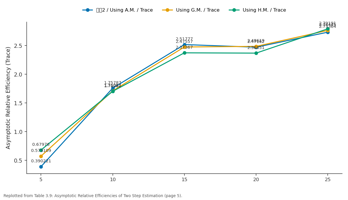
ൌ2 / Using A.M. / Trace and Using G.M. / Trace and more: 5 vs 10 vs 15 vs 20 vs 25
Replotted from Table 3 (page 5) of the original paper. Every bar is the paper's own table value.
View source evidence ↗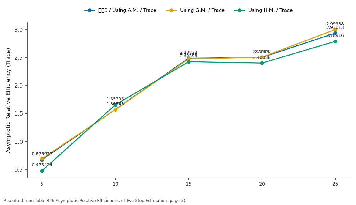
ൌ3 / Using A.M. / Trace and Using G.M. / Trace and more: 5 vs 10 vs 15 vs 20 vs 25
Replotted from Table 3 (page 5) of the original paper. Every bar is the paper's own table value.
View source evidence ↗Figures & tables
From the original paper Table 2
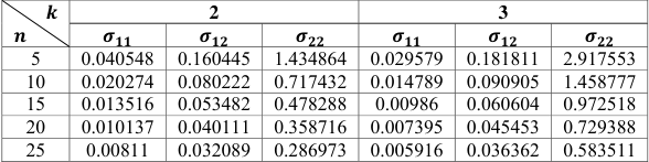 Table 2
 Table 3
 Table 3
 Table 3
 Table 3
 Table 3
 Table 3
 Table 3
 Table 3
 Table 3
 Table 3
Introduction
In reliability studies exponential distribution is the central model for the study of any phenomenon through a probabilistic approach. Extension of this model into two different directions yields two popular models called the Weibull distribution and the gamma distribution. Between these two, the Weibull distribution is more frequently applied model in any practical situation concerning reliability studies. Both Weibull and gamma distributions involve a shape parameter, in the sense that the shape of the frequency curve of these models changes according as the change in the values of the shape parameters. In particular, for the Weibull distribution its shape parameter classifies it into an Increasing Failure Rate (IFR) model or a Decreasing Failure Rate (DFR) model or Constant Failure Rate (CFR) model (the well-known exponential model) as its special cases. The natural phenomenon in reliability is "The aging concept" -indicated by increasing instantaneous failure probability with age of the product. A specific case of Weibull distribution exhibiting aging effect with an integer valued shape parameter is known as "The Rayleigh distribution". Its cumulative distribution function (CDF), probability density function (PDF) and hazard function are given by 1 (1.1)
is the cumulative distribution function of a positive valued random variable, then , k>0 also satisfies all the requirements for the cumulative distribution function of another positive valued random variable. It can be interpreted as the failure probability of a parallel system of k-components whose life times are independently and identically distributed random variables, each with a common CDF -F(x) if k is an integer. Exploring this concept to non-integer values of k also, many researchers in the recent past made extensive studies on models of the type generated by a basic well known model F(x). Such new models are named as exponentiated models by some authors and generalised models by some authors. For instance if the basic F(x) is exponential, is named as generalised exponential (Gupta & Kundu-1999) [3] , if F(x) is Weibull, is named as exponentiated Weibull (Mudholkar and Srivastava -1993). Banking on this notion, generalised Rayleigh distribution was studied by Raqab and Kundu (2006) [5] , as a process of revisit to Burr type X distribution. Its cumulative distribution function (CDF), probability density function (PDF) and hazard function are given by ;
Burr (1942) [1] has suggested a number of forms of cumulative distribution functions that might be useful in modeling various practical situations. In all, he suggested twelve models as listed below. Thus generalised Rayleigh distribution and Burr type X distributions are one and the same.
In the above models k and c are the positive parameters involved in the respective models. The first model is the well-known uniform distribution also included by Burr (1942) [1] . Among these twelve forms, the type X and type XII models are most frequently applied by many researchers. Our focus is Burr Type X model, whose expressions are given in equations (1.4), (1.5), and (1.6). If a scale parameter say λ is introduced, the cumulative distribution function, probability density function and hazard function are given by ; ,
Expressions in (1.4), (1.5) and (1.6) are called standard Burr type X model, those in equations (1.8), (1.9) and (1.10) are called scaled Burr type X or Two parameter Burr type X model. In this paper estimation of parameters of the Burr type X model is studied. Though this is attempted by other researchers in the past (Kundu and Raqab-2005 and the references therein) [6] our approach of estimation is different from theirs. We consider the two parameter Burr X distribution one of which is its scale parameter and the other is its shape parameter. We first take up the well-known classical maximum likelihood method of estimation of the parameters from complete sample when both the parameters are unknown. In view of the iterative nature of the solutions of the log likelihood equations, we make a modest beginning of estimating one of the parameters when the other is known. For the classical maximum likelihood estimation approach for both the parameters we derive the elements of the information matrix, asymptotic dispersion matrix, and their computed values in Section -2 as these are rarely available in published form. We estimate both the parameters λ and k of Burr type X distribution by using Two Step Estimation method. The asymptotic relative efficiency of two step estimation results are presented in relation to empirical dispersion matrix, asymptotic dispersion matrix in Section -3.
Maximum Likelihood Estimation
The probability density function of the two parameter Burr type X distribution is given by ; , 2 1 ; 0, 0, 0 (2.1) Let x1<x2<x3<…<xn be a complete ordered sample of size n drawn from the above distribution (Though for complete samples maximum likelihood estimation does not require ordering of the sample, in order to facilitate presenting the methods to be introduced in Section -3 which depend on ordered samples we consider ordered complete samples in the beginning itself, for uniformity in the notation.). The log likelihood equations to get the maximum likelihood estimates of λ and k are given by (after simplification).
3) These equations show that maximum likelihood estimator of λ is an iterative solution involving k and maximum likelihood estimator of k is a closed form expression involving λ given as
Since λ is a scale parameter, in view of the scale invariant nature of the Burr type X distribution, maximum likelihood estimation of k can be taken as the following expression in a standard model.
where . The elements of the information matrix and hence those of the asymptotic dispersion matrix require the following second order partial derivatives. As the integrals involved in these mathematical expectations are not analytically tractable we have evaluated them using 11-point Gauss-Laguerre quadrature formula (Rao et al., 1966) [7] for selected values of k in a standard density (λ=1) and are given in Table -
Two Step Estimation Procedure of Burr Type X Distribution
In this Section we discuss the point estimation of both the parameters λ and . We notice that the log likelihood equations to get the MLEs of λ and as presented in Section -2 yield an analytical expression for the MLE of whereas an iterative solution for λ. We suggest different methods of estimation for λ and based on the same sample in order to get their estimates finally on the basis of a given sample. Such a procedure is called Two Step Estimation as done by Engeman and Keefe (1985) [2] for the Weibull distribution, Srinivasa Rao and Kantam (2012) [8] for log logistic distribution and the references there in. In the present situation we estimate λ as described below.
Consider the CDF of the two parameter Burr type X given by 1 (3.1) Let , be two observations from this CDF with . Let be two real numbers between 0 and 1such that, . Consider the two following equations
Taking logarithms and dividing we get If we have a random sample of size more than 2 ( 3) we propose the following procedure in order to use all the observations to get as given in equation (3.5). We order the sample of n observations in ascending manner and divide it into two halves -lower half and upper half of 2 n observations each, deleting the sample median in case the sample size is odd. We consider the arithmetic means of observations in lower half and upper half as , respectively for use in the formula (3.5). This procedure uses all the sample observations but one to estimate λ if the sample size is greater than are equal to 4. We call this way of estimating λ as the first step of estimation. The estimate of λ so obtained in the first step shall then be used in the expression for the exact MLE of k given by ∑ .
When both the parameters are unknown we suggest to estimate λ in the first step of estimation by dividing the ordered sample as lower and upper halves to make use of the formula (3.5). As a matter of academic interest, we suggest to use the arithmetic means AM , AM , geometric means GM , GM and harmonic means HM , HM of the two halves of the divided ordered sample in succession in the place of x1, x2 of equation (3.5).
Next, in the second step of estimation, the parameter k is estimated by the exact ML method given by the formula (3.6) together with the estimate of λ obtained in the first step of estimation. We name this entire procedure as two step estimation -a hybrid of an adhoc method and an exact ML method. The performance of such a two-step procedure is studied in the following lines through Monte -Carlo simulation by computing the empirical variance covariance matrix of , for n=5(5)25, k=2, 3, where is given by (3.5) and is given by (3.6) over 10,000 runs. Results are presented in Tables 3.1 through 3.6.
For the sake of comparison with the asymptotic dispersion matrix of MLEs of , , we present those elements also in Tables 3.7 and 3.8 for k= 2, 3. The trace, the determinant of the dispersion matrices called the generalised variances in the multi parameter case are also given in the respective tables. The ratios of the determinant of the asymptotic dispersion matrix from Tables 3.7 and 3.8 to the corresponding value of the determinant of the empirical dispersion matrix of the two step estimators for n=5(5)25, k= 2, 3 are given in Table -3.9 naming them as Asymptotic Relative Efficiencies (ARE) of the two step estimation with respect to determinant of dispersion matrix as a generalised variance. Similarly, the ratios of trace of the asymptotic dispersion matrix to the corresponding trace of empirical dispersion matrix of the two step estimators are also given in Table -3.9 as another measure of ARE with respect to another generalised variance. We see from Table -3.9 that the suggested two step estimation is performing very encouragingly with the ARE more than one in most of the cases.
Figures and tables from the paper
| | 2 | — | — | 3 | — | — |
|---|---|---|---|---|---|---|
| Matrix | I11 | I12 | I22 | I11 | I12 | I22 |
| 8.84668 | -0.989225 | 0.25 | 10.9596 | -0.68296 | 0.1111 |
Table text extracted from the original PDF; superscript letters are shown inline. The original table image is below.
View original table image
| | 2 | — | — | 3 | — | — |
|---|---|---|---|---|---|---|
| ࣌ | ࣌ | ࣌ | ࣌ | ࣌ | ࣌ | |
| 5 | 0.040548 | 0.160445 | 1.434864 | 0.029579 | 0.181811 | 2.917553 |
| 10 | 0.020274 | 0.080222 | 0.717432 | 0.014789 | 0.090905 | 1.458777 |
| 15 | 0.013516 | 0.053482 | 0.478288 | 0.00986 | 0.060604 | 0.972518 |
| 20 | 0.010137 | 0.040111 | 0.358716 | 0.007395 | 0.045453 | 0.729388 |
| 25 | 0.00811 | 0.032089 | 0.286973 | 0.005916 | 0.036362 | 0.583511 |
Table text extracted from the original PDF; superscript letters are shown inline. The original table image is below.
View original table image
| | ࢂ൫ࣅ൯ | ࢂ൫൯ | ࢜൫ࣅ, ൯ | Determinant of the Matrix | Trace of the Matrix |
|---|---|---|---|---|---|
| 5 | 0.05055 | 3.730416 | 0.311044 | 0.091824 | 3.780966 |
| 10 | 0.020419 | 0.39924 | 0.088655 | 0.000292 | 0.419659 |
| 15 | 0.011113 | 0.18422 | 0.044888 | 3.23E-05 | 0.195333 |
| 20 | 0.00886 | 0.140375 | 0.03507 | 1.38E-05 | 0.149235 |
| 25 | 0.00643 | 0.101515 | 0.025387 | 8.24E-06 | 0.107945 |
Table text extracted from the original PDF; superscript letters are shown inline. The original table image is below.
View original table image
| | ࢂ൫ࣅ൯ | ࢂ൫൯ | ࢜൫ࣅ, ൯ | Determinant of the Matrix | Trace of the Matrix |
|---|---|---|---|---|---|
| 5 | 0.046699 | 4.326304 | 0.417914 | 0.027382 | 4.373003 |
| 10 | 0.017762 | 0.920913 | 0.124873 | 0.000764 | 0.938675 |
| 15 | 0.009864 | 0.384948 | 0.060987 | 7.77E-05 | 0.394812 |
| 20 | 0.007331 | 0.287159 | 0.045482 | 3.66E-05 | 0.29449 |
| 25 | 0.005496 | 0.195254 | 0.032597 | 1.06E-05 | 0.20075 |
Table text extracted from the original PDF; superscript letters are shown inline. The original table image is below.
View original table image
| | ࢂ൫ࣅ൯ | ࢂ൫൯ | ࢜൫ࣅ, ൯ | Determinant of the Matrix | Trace of the Matrix |
|---|---|---|---|---|---|
| 5 | 0.051894 | 2.522506 | 0.303581 | 0.038742 | 2.5744 |
| 10 | 0.019667 | 0.411583 | 0.087936 | 0.000362 | 0.43125 |
| 15 | 0.011554 | 0.187109 | 0.046195 | 2.79E-05 | 0.198663 |
| 20 | 0.008636 | 0.139725 | 0.034567 | 1.18E-05 | 0.148361 |
| 25 | 0.006321 | 0.100421 | 0.025048 | 7.36E-06 | 0.106742 |
Table text extracted from the original PDF; superscript letters are shown inline. The original table image is below.
View original table image
| | ࢂ൫ࣅ൯ | ࢂ൫൯ | ࢜൫ࣅ, ൯ | Determinant of the Matrix | Trace of the Matrix |
|---|---|---|---|---|---|
| 5 | 0.045026 | 4.213351 | 0.396786 | 0.032271 | 4.258377 |
| 10 | 0.016873 | 0.923231 | 0.121203 | 0.000888 | 0.940104 |
| 15 | 0.009454 | 0.387436 | 0.059963 | 6.73E-05 | 0.39689 |
| 20 | 0.007368 | 0.286587 | 0.045558 | 3.6E-05 | 0.293955 |
| 25 | 0.00557 | 0.190946 | 0.032445 | 1.09E-05 | 0.196516 |
Table text extracted from the original PDF; superscript letters are shown inline. The original table image is below.
View original table image
| | ࢂ൫ࣅ൯ | ࢂ൫൯ | ࢜൫ࣅ, ൯ | Determinant of the Matrix | Trace of the Matrix |
|---|---|---|---|---|---|
| 5 | 0.051899 | 2.11859 | 0.293146 | 0.024018 | 2.170489 |
| 10 | 0.021184 | 0.412044 | 0.092278 | 0.000214 | 0.433228 |
| 15 | 0.011424 | 0.195767 | 0.046908 | 3.61E-05 | 0.207191 |
Table text extracted from the original PDF; superscript letters are shown inline. The original table image is below.
View original table image
| | ࢂ൫ࣅ൯ | ࢂ൫൯ | ࢜൫ࣅ, ൯ | Determinant of the Matrix | Trace of the Matrix |
|---|---|---|---|---|---|
| 5 | 0.044031 | 6.154925 | 0.433282 | 0.083274 | 6.198956 |
| 10 | 0.017684 | 0.873569 | 0.122188 | 0.000518 | 0.891253 |
| 15 | 0.009821 | 0.39546 | 0.061372 | 0.000117 | 0.405281 |
| 20 | 0.007642 | 0.299302 | 0.047438 | 3.69E-05 | 0.306944 |
| 25 | 0.005445 | 0.205883 | 0.033295 | 1.25E-05 | 0.211328 |
Table text extracted from the original PDF; superscript letters are shown inline. The original table image is below.
View original table image
| | ࣌ | ࣌ | ࣌ | Determinant of the Matrix | Trace of the Matrix |
|---|---|---|---|---|---|
| 5 | 0.040548 | 1.434864 | 0.160445 | 0.032438 | 1.475412 |
| 10 | 0.020274 | 0.717432 | 0.080222 | 0.00811 | 0.737706 |
| 15 | 0.013516 | 0.478288 | 0.053482 | 0.003604 | 0.491804 |
| 20 | 0.010137 | 0.358716 | 0.040111 | 0.002027 | 0.368853 |
| 25 | 0.00811 | 0.286973 | 0.032089 | 0.001298 | 0.295083 |
Table text extracted from the original PDF; superscript letters are shown inline. The original table image is below.
View original table image
| | ࣌ | ࣌ | ࣌ | Determinant of the Matrix | Trace of the Matrix |
|---|---|---|---|---|---|
| 5 | 0.029579 | 2.917553 | 0.181811 | 0.053243 | 2.947132 |
| 10 | 0.014789 | 1.458777 | 0.090905 | 0.01331 | 1.473566 |
| 15 | 0.00986 | 0.972518 | 0.060604 | 0.005916 | 0.982378 |
| 20 | 0.007395 | 0.729388 | 0.045453 | 0.003328 | 0.736783 |
| 25 | 0.005916 | 0.583511 | 0.036362 | 0.00213 | 0.589427 |
Table text extracted from the original PDF; superscript letters are shown inline. The original table image is below.
View original table image
| | ൌ2 | — | — | — | — | — | ൌ3 | — | — | — | — | — |
|---|---|---|---|---|---|---|---|---|---|---|---|---|
| Using A.M. | Using G.M. | Using H.M. | Using A.M. | Using G.M. | Using H.M. | |||||||
| Trace | Determ- inant | Trace | Determ- inant | Trace | Determ- inant | Trace | Determ- inant | Trace | Determ- inant | Trace | Determ- inant | |
| 5 | 0.390221 | 0.353263 | 0.573109 | 0.837283 | 0.67976 | 1.35057 | 0.673938 | 1.944453 | 0.692079 | 1.649871 | 0.475424 | 0.639371 |
| 10 | 1.75787 | 27.77397 | 1.710623 | 22.40331 | 1.702812 | 37.8972 | 1.569836 | 17.42147 | 1.56745 | 14.98874 | 1.653364 | 25.69498 |
| 15 | 2.517772 | 111.5789 | 2.475569 | 129.1756 | 2.373675 | 99.8338 | 2.488217 | 76.139 | 2.47519 | 87.9049 | 2.423943 | 50.5641 |
| 20 | 2.471625 | 146.8841 | 2.486186 | 171.7797 | 2.368511 | 87.37069 | 2.501895 | 90.92896 | 2.506448 | 92.44444 | 2.400382 | 90.1897 |
| 25 | 2.733642 | 157.5243 | 2.764451 | 176.3587 | 2.791914 | 329.4416 | 2.936125 | 200.9434 | 2.999384 | 195.4128 | 2.789157 | 170.4 |
Table text extracted from the original PDF; superscript letters are shown inline. The original table image is below.
View original table image
References
8 in the original paper- Burr IW. Cumulative Frequency Functions. The Annals of Mathematical Statistics. 1942; 13:215-232.
- Engeman PR, Keefe TJ. Two-Step Estimators of the Scale Parameters of the Weibull Distribution. Computers and Biomedical Research. 1985; 18:391-396.
- Gupta RD, Kundu D. Generalized Exponential Distributions. Australian and New Zealand Journal of Statistics. 1999; 41(2):173-188.
- Mudholkar Govind S, Srivastava Deo Kumar. Exponentiated Weibull family for analyzing bathtub failure-rate. Reliability, IEEE Transaction. 1993; 42(2):299-302.
- Raqab MZ, Kundu D. Burr type X distribution: revisited. Journal of Probability and Statistical Science. 2006; 8:179-198.
- Kundu D, Raqab MZ. Generalized Rayleigh Distribution: Different Methods of Estimation. Computational Statistics & Data Analysis. 2005; 49:187-200.
- Rao CR, Mathai A, Mitra SK. Formulae and Tables for Statistical Work. Statistical Publishing Society, Calcutta, India, 1966, 162.
- Srinivasa Rao G, Kantam RRL. Two-Stage Estimation in log-logistic Model. Pakistan Journal of Statistics. 2012; 28(3):331339.
Cited by 1
From OpenAlex, OpenCitations and reference lists read by Scinovex
- DAGUM DISTRIBUTION-A TWO STEP PARAMETRIC ESTIMATION ↗
B. Srinivasa Rao, P. Sricharani · Journal of Statistics Advances in Theory and Applications · 2018
The three parameter Dagum distribution is considered.The well known classical method -maximum likelihood (ML) estimation of three parameters is used which resulted in iterative solutions of the parameters.Hence, we propose a more efficient and computationally simple/analytical estimation procedure called two-step estimation.Using real data sets the procedure illustrated.
❝ 0PDF