
Research article · 2017 · Full text
International Journal of Statistics and Applied MathematicsA multivariate analysis approach in determining potential hotspots of seasonal rainfall change over Uganda
Volume 2(1) · Pages 31–41
Research areasHydrology and Drought AnalysisClimate change impacts on agricultureComputational Physics and Python Applications
Abstract
Author-writtenEvidence of climate change continues to emerge in Uganda as indicated by recent floods in Teso sub-region and Kasese district, landslides in Bududa and long droughts experienced in Karamoja. The major objective of the study was to identify potential hotspots of rainfall change in Uganda during March-May and October-December seasons. Monthly rainfall data for the period extending from 1951 to 2010 were used in the study. ArcGIS, a geographic information system tool was used to determine geographical areas that have experienced changes in seasonal rainfall over the decades 1981-2010 relative to the long-term mean (1951-2010). Mbale, Mbarara and Moroto were identified as areas of potential rainfall change. The historical rainfall series for the identified areas were tested for inhomogeneities using Standard Normal Homogeneity and Pettitt tests and found to be homogenous. Multivariate two-sample Hotelling T2-test was used to generate evidence of rainfall change in the identified areas by comparing mean seasonal rainfall vectors between the sub-periods 1951-1980 and 1981-2010. Results indicated a significant simultaneous decrease in mean rainfall over Moroto and Mbarara areas across the March-May season with April having the highest decrease (11 mm and 18 mm respectively). Mean rainfall in Mbale was found to have increased simultaneously across both wet seasons with April and October experiencing the greatest increase (10 mm apiece). These changes have detrimental effects on crop and livestock farming as well as human lives. There is need for increased climate change adaptation and resilience action in the identified areas through up-scaling of climate smart agricultural interventions.
Summary
Source-checkedPlain-language reading of the full paper, prepared with AI and checked against the text. Each point links to the authors' own words.
Why it matters
- Uganda is highly susceptible to climate change because most of its people rely on rain-fed agriculture for their livelihoods. View evidence ↗
- Recent environmental events in Uganda, including floods in Kasese and Teso, landslides in Bududa, and droughts in Karamoja, provide evidence of ongoing climate change. View evidence ↗
- Standard univariate climate trend analyses are insufficient for understanding seasonal changes because a rainfall season consists of multiple monthly variables. View evidence ↗
The question
- The study aimed to identify potential hotspots of rainfall change in Uganda specifically during the March-May and October-December seasons. View evidence ↗
What they did
- The researchers analyzed monthly rainfall data spanning the years 1951 to 2010. View evidence ↗
- ArcGIS was employed to map areas where seasonal rainfall from 1981-2010 deviated from the long-term mean of 1951-2010. View evidence ↗
- A multivariate two-sample Hotelling T2-test compared mean seasonal rainfall vectors between the 1951-1980 and 1981-2010 sub-periods to identify significant changes. View evidence ↗
- Mbale, Mbarara, and Moroto were selected as the primary areas for detailed analysis of rainfall change hotspots. View evidence ↗
What they found
- The historical rainfall data for the selected hotspot areas were confirmed to be homogeneous using SNHT and Pettit tests. View evidence ↗
- In Mbale, mean rainfall increased across the March-May (MAM) season, with the most significant increase of approximately 10 mm occurring in April. View evidence ↗
- During the MAM season, mean rainfall decreased in Mbarara and Moroto, with April seeing the largest drops of 18 mm and 11 mm, respectively. View evidence ↗
- For the October-December (OND) season, only Mbale showed a significant increase in rainfall across all months, with October increasing by about 10 mm. View evidence ↗
- No significant difference in mean rainfall vectors was found for Mbarara and Moroto during the OND season when comparing the two sub-periods. View evidence ↗
What it means
- The authors concluded that Moroto and Mbarara are hotspots for rainfall decrease (primarily in MAM), while Mbale is a hotspot for rainfall increase in both wet seasons. View evidence ↗
- The authors recommend focusing climate adaptation efforts in these hotspots through investments in climate-smart agriculture, such as water harvesting and improved crop varieties. View evidence ↗
- The authors state a need for future work to distinguish between hotspots in unimodal and bimodal rainfall regimes to account for regional disparities in northern Uganda. View evidence ↗
Visual summary
1 visualsIllustrations explain the paper; they do not show study data.
Rainfall Hotspot Summary
AI-generated conceptual illustration (A map of Uganda with regional weather indicators). It explains the idea and does not show study data.
View source evidence ↗Figures & tables
From the original paper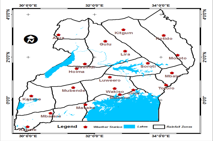 Figure 1
 Table 1
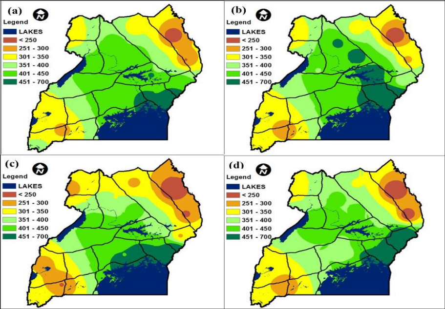 Figure 2
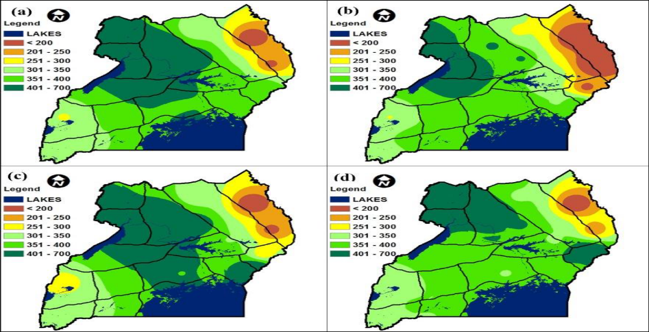 Figure 3
 Table 2
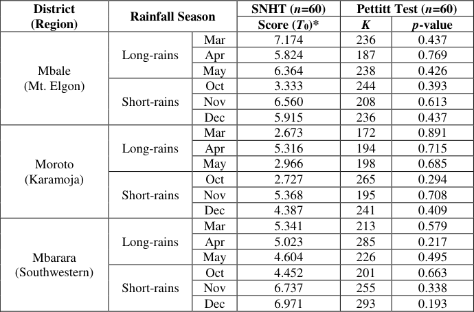 Table 3
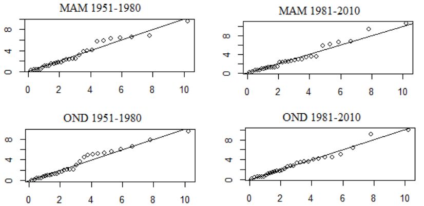 Figure 4
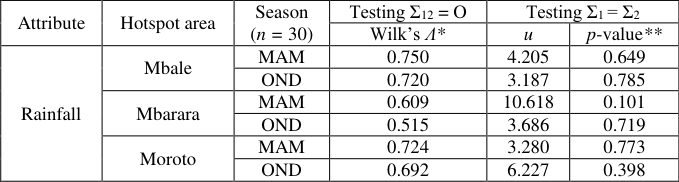 Table 4
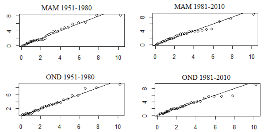 Figure 4
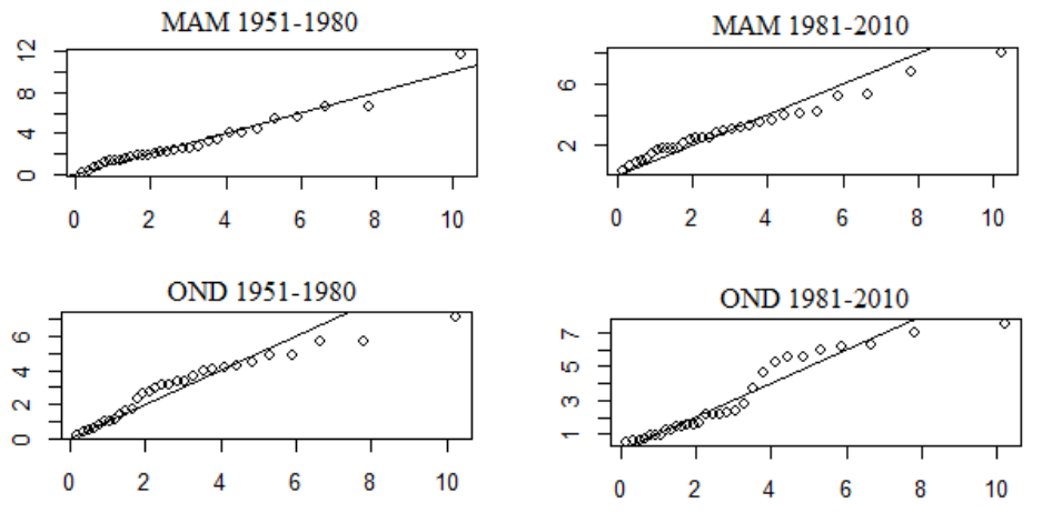 Figure 4
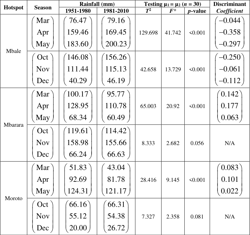 Table 5
Introduction
Evidence of climate change around the globe is emerging through increase in rainfall variability and the frequency of extreme weather events such as drought, floods and hurricanes, all which are very likely to be associated with the observed increase in anthropogenic greenhouse gas emissions (Intergovernmental Panel on Climate Change IPCC, 2007). Climate change hotspots have been defined by Thornton et al., (2008) [2] as regions that are particularly at risk of suffering significant impacts from current or future climate change. This encompasses geographic areas projected to experience relatively large changes in temperatures and rainfall amounts and patterns. Hagenlocher et al., (2014) [5] defines hotspots as areas where extreme flood and drought events have occurred more frequently over the past three decades and trends in rainfall and temperature are evident, particularly during the wet seasons. Uganda is one of the developing countries grappling with the impacts of climate change and variability as indicated by recent floods in Teso sub region and Kasese district, landslides in Bududa and long droughts experienced in the Karamoja; all of which have led to crop loss and subsequent famine and displacement of people (Government of Uganda GOU, 2010). As such, Uganda is vulnerable to climate change since majority of its population derive their livelihood from rain-fed agriculture (Mukiibi, 2001) [13] .
According to Phillips and McIntyre (2000) [20] , Uganda experiences two major rainfall regimes namely bimodal and unimodal. The bimodal regime is observed over majority of the country such as the southern region and areas near the equator with the first wet season occurring in March-May (MAM), also known as 'long-rains'. The second wet season takes place in October-December (OND) and is also known as 'short-rains'. The unimodal pattern on the other hand dominates areas far north of Uganda where the two wet seasons merge forming one long wet season from April-September. Oxfam (2008) [18] reported that farmers in Uganda observe an increasingly inconsistent rainfall pattern in the MAM season often resulting into drought and crop failure, but also more extreme rainfall during the OND season at the end of the year, causing flooding and erosion. Local level studies conducted in Uganda to provide evidence of changing climate have focused mostly on trends in daily, monthly, seasonal and annual rainfall (Ogwang et al., 2012; Mubiru et al., 2012; Nsubuga et al., 2014; Kansiime et al., 2013; Kizza et al., 2009; Stampone et al., 2011; Diem et al., 2014; Osbahr et al., 2011) [16,12,15,8,10,22,3,17] . Majority of these reveal that rainfall has significantly declined in the cattle corridor axis (stretching from the Karamoja region in the Northeast, through Central, down to the Ankole region in the Southwest); conversely, an increase in rainfall is evident in Eastern Uganda (Mt. Elgon region) and parts of Lake Victoria basin. Climatic trends are limited to describing patterns in only univariate data, yet a rainfall season is defined by observations from more than one variable (month). As such, climate trend analyses yield little information about changes in rainfall seasons over time. This study addressed the gap by using spatial analysis as well as multivariate analysis techniques on historical rainfall data to simultaneously examine changes across the major rainy seasons, as a way of providing evidence of rainfall change over Uganda.
This study has identified the potential hotspots of rainfall change over Uganda with focus on March-May (MAM) and October-December (OND) seasons. We have determined the geographic areas in Uganda whose seasonal rainfall over the past three decades (1981-2010) deviates from the long-term mean. Data quality control was undertaken on the acquired historical rainfall data for the identified areas. Finally, we carried out detailed statistical analysis on the historical datasets to determine evidence of rainfall change in the identified areas.
Methodology
Uganda lies in East Africa, astride the equator with its area lying between latitude 4 0 12'N and 1 0 29'S and longitude 29 0 34'W and 35 0 0'E. It has an estimated total area of 241,040 Km 2 and its altitude ranges between 620 m (Albertine Rift) and 5110 m (Mt. Rwenzori), with a mean of 1200 m above sea level. Uganda's climate is typically tropical with moderate variation in temperature throughout the year. Uganda has five climatic zones, which include: the Lake Victoria basin, the Karamoja region, Western Uganda, the Acholi-Kyoga region and the Ankole-southern area. Distinctive wet and dry seasons characterize most of the country's climate, except in the semi-arid northeast. Annual rainfall and temperature range from 700 mm to 3000 mm; and 16 0 C to 31 0 C, respectively and show variation depending on elevation and landscape (NEMA, 2010) [14] . Monthly rainfall records for selected meteorological stations (Figure 1) across Uganda for the period extending from 1951 to 2010 were used in this study. The data were acquired from Uganda National Meteorological Authority (UNMA) database. The stations used were selected basing on data availability and representation of the homogenous rainfall zones defined by Basalirwa (1995) [2] . Gaps in existing historical weather data alluding to stolen or old equipment and shortage of trained observers confounds climate change related analyses. This problem was addressed by filling the gaps using satellite-based observations and automated weather data in line with suggestions by Komutunga et al., (2015) [11] . Modern-Era Retrospective Analysis for Research and Applications (MERRA) satellite data at 0.25 degree resolution were acquired from the National Aeronautics and Space Administration (NASA), while automated weather data were obtained from Adcon telemetry database of the National Agricultural Research Organization (NARO). The satellite/automated data were adjusted for differences in location and time of observation and then compared to manual (station) records using linear regression methods. Locations whose observations correlated strongest with actual data were then used to estimate the missing data. [2] from which the stations used in the study were selected Long-term mean for each rainfall season was computed by averaging total rainfall observations over the entire study period (1951-2010). Deviations from long-term mean rainfall totals during the major rainy seasons for the decades 1981-1990, 1991-2000 and 2001-2010 were mapped using ArcGIS, a geographic information system (GIS) tool tailored for spatial analysis. The main problem with time series from station data is that they are often not homogeneous as they exhibit trends or sudden jumps in the mean or variance. This may be caused by changes in the: observing site, observing equipment, observing procedures and time, and personnel. Any conclusions drawn from analyzing such data may thus be biased (von Storch and Zwiers, 2001) [24] . In this study, two methods were used to detect departures from homogeneity in the rainfall series for the identified areas: namely Standard Normal Homogeneity Test (SNHT) for a single break and Pettit test. These two tests are capable of locating the time (year) where a break is likely. The SNHT detects breaks near the beginning and the end of a series relatively easily, whereas the Pettit test is more sensitive to breaks in the middle of a time series (Wijngaard et al., 2003) [25] . The following hypotheses on homogeneity were tested: H0: The values xi of the testing variable X are homogenous HA: A step-wise shift in the mean (a break) is present Alexandersson (1986) describes a statistic T(k) for detecting a shift in the mean value of a time-series by comparing the mean of the first k years of the record with that of the last nk years:
Data Analysis Standard Normal Homogeneity Test (SNHT)
(2) where 𝑋 ̅ and s are the estimated mean and standard deviation of observations xi respectively. If a break is located at the year K, then T(k) reaches a maximum near the year k = K. This is depicted in the graphs representing the results of this test. The test statistic T0 is defined as:
The null hypothesis H0 is rejected if T0 is above a certain level, which is dependent on the sample size as shown by the critical values in Table 1.
| N | 20 | 30 | 40 | 50 | 60 | 70 | 100 |
|---|---|---|---|---|---|---|---|
| T95 | 7.089 | 7.747 | 8.151 | 8.432 | 8.647 | 8.814 | 9.167 |
| T99 | 9.113 | 10.153 | 10.771 | 11.193 | 11.498 | 11.737 | 12.228 |
Table text extracted from the original PDF; superscript letters are shown inline. The original table image is below.
View original table image
Pettitt Test
This approach by Pettitt (1979) is commonly applied to detect a single change-point in a time-series with continuous data. For T observations, the test statistic is defined as:
The change-point of the series is located at t, provided that the statistic is significant. Evidence of rainfall change in the identified areas was determined by making simultaneous comparison of mean seasonal rainfall between two sub-periods of time. The sub-periods compared were each of length thirty years, in line with the recommended minimum baseline period for climatological assessments by the World Meteorological Organization (WMO, 1996). A multivariate analysis approach was used where each rainfall season was assumed to constitute p x 1 and q x 1 random vectors representing the first and second sub-periods (groups) respectively. The variables measured on each unit (year of observation) were total rainfall in Mar, Apr and May or Oct, Nov and Dec. Since each rainfall season is made up of three months, it implies that p = q = 3, thus yielding a three-variate data structure as illustrated below: Let y be an observation vector containing monthly total rainfall of a single rainfall season for the two sub-periods to be compared:
where y1 and y2 are sub-vectors (each of dimension 3 x 1) representing the months of a particular rainfall season in the first and second sub-periods respectively.
Multivariate Two-sample Hotelling T 2 test
The rainfall mean vectors defining MAM and OND seasons were compared between two sub-periods of time using Multivariate Two-Sample Hotelling's T 2 -test (Hotelling, 1951), a special case of the One-way Multivariate Analysis of Variance (MANOVA) model. The statistical differences between the mean vectors were tested as described below by Rencher (2003) [21] . The Hotelling's T 2 -test assumes that (i)
In each population, the variables have a multivariate normal distribution, (ii) the observations are independent in each population, and (iii) the populations have the same covariance matrix Assumption (i) was checked using chi-square plots of standardized distances
where yi is the data vector containing seasonal rainfall observations for a particular sub-period, 𝐲 ̅ is the sample mean vector and S is the sample covariance matrix. A non-linear pattern in the plot would indicate a departure from multivariate normality while points close to a straight line indicate no deviation from the assumption. Assumption (ii) was tested by checking the independence of two sub-vectors. Suppose the observation vector y is partitioned into two sub-vectors of interest y1 and y2 of dimension p × 1 and q x 1 respectively, as shown in equation ( 6). The corresponding partitioning of the population and sample covariance matrices is
The hypothesis of independence of sub-vectors y1 and y2 can be expressed as 01 12 11 12 vs.
which means that every variable in y1 is independent of every variable in y2. The likelihood ratio test statistic for H01 is given by
which is distributed as , ,
The critical values for Wilks' Ʌ at 5% significance level were obtained from Rencher (2003) [21] . : :
Assumption (iii) was tested as follows:
Assuming independent samples of size n1 and n2 from multivariate normal populations, and defining the corresponding degrees of freedom as v1 and v2, the test statistic u is computed by chi-square approximation as follows:
S
The null hypothesis H02 is rejected if 2 0.05 u or if the p-value < 0.05. Having affirmed that the data are independent, multivariate normal and that the covariance matrices are equal, the hypothesis for equality of mean vectors was then tested as shown below:
Assuming the first sub-period of time forms a random sample , N μ Σ the first step is to compute the sample mean vectors:
respectively, they can be pooled to obtain an unbiased estimator Sp of the common population covariance matrix Σ:
S S S (15)
The multivariate two-sample Hotelling's T 2 -statistic is obtained as:
y y S y y (16) which is distributed as
The Multivariate Two-Sample Hotelling's T 2 -test is a special case of the One-way MANOVA model, where population mean vectors of two groups (k = 2) are compared. Following this relationship, the Hotelling T 2 -statistic can be transformed to an approximate F-statistic as follows
At 5% significance level, H03 is rejected if
or if p < 0.05. Suppose that the Hotelling T 2 -test leads to the rejection of H03, the discriminant function coefficient vector a is computed in order to determine the individual variables (months) that contribute most to separation of the two groups (sub-periods) Contrary to the MAM season, rainfall during the OND season showed no drastic changes from its long-term mean for majority of the country. However, rainfall increments (over 400 mm) during this season are evident in Eastern Uganda particularly around Mt. Elgon area (Figure 3).
Selected areas for further analysis of hotspots of rainfall change
Following the spatial analysis results of changes in seasonal rainfall over Uganda as presented by Figures 2 and3, areas that showed notable departure from long-term mean rainfall were selected for further investigation in order to provide evidence of change. Table 2 gives a brief description of meteorological stations that were used for this task.
| Station name | District | Latitude (decimal 0) | Longitude (decimal 0) | Elevation (m) | Region |
|---|---|---|---|---|---|
| Mbale forest station | Mbale | 1.267 | 34.350 | 1875 | Eastern (Mt. Elgon) |
| Nabilatuk Station | Moroto | 2.100 | 34.517 | 1250 | Northeastern (Karamoja) |
| Mbarara Met Station | Mbarara | -0.617 | 30.683 | 1420 | Southwestern |
Table text extracted from the original PDF; superscript letters are shown inline. The original table image is below.
View original table image
Quality control on historical rainfall data for the identified areas
Historical rainfall datasets for the stations representing the identified hotspot areas were tested for inhomogeneities and found to be homogeneous by both SNHT and Pettit tests (Table 3). The computed values from the SNHT statistic were all less than the critical value (8.647) while the p-values from Pettitt test were greater than 0.05, thus providing no sufficient evidence against the assumption of homogeneity. The data were therefore fit to be used for further statistical analyses. The chi-square plots for MAM and OND seasons over Mbale and Mbarara areas showed no notable deviations from linearity (Figures 4(a) and4(b)). This implied that the total rainfall for the months defining each season followed a multivariate normal distribution in each sub-period. For cases where the assumption of multivariate normality was violated such as OND rainfall in Moroto, Hotelling T 2 and MANOVA were still applied since these tests have been found to be fairly robust to departures from multivariate normality and heterogeneity of covariance matrices as long as the sample sizes are large and equal (Rencher, 2003) [21] .
| District (Region) | Rainfall Season | — | SNHT (n=60) | Pettitt Test (n=60) | — |
|---|---|---|---|---|---|
| Score (T0)* | K | p-value | |||
| Mbale (Mt. Elgon) | Long-rains | Mar | 7.174 | 236 | 0.437 |
| Apr | 5.824 | 187 | 0.769 | ||
| May | 6.364 | 238 | 0.426 | ||
| Short-rains | Oct | 3.333 | 244 | 0.393 | |
| Nov | 6.560 | 208 | 0.613 | ||
| Dec | 5.915 | 236 | 0.437 | ||
| Moroto (Karamoja) | Long-rains | Mar | 2.673 | 172 | 0.891 |
| Apr | 5.316 | 194 | 0.715 | ||
| May | 2.966 | 198 | 0.685 | ||
| Short-rains | Oct | 2.727 | 265 | 0.294 | |
| Nov | 5.368 | 195 | 0.708 | ||
| Dec | 4.387 | 241 | 0.409 | ||
| Mbarara (Southwestern) | Long-rains | Mar | 5.341 | 213 | 0.579 |
| Apr | 5.023 | 285 | 0.217 | ||
| May | 4.604 | 226 | 0.495 | ||
| Short-rains | Oct | 4.452 | 201 | 0.663 | |
| Nov | 6.737 | 255 | 0.338 | ||
| Dec | 6.971 | 293 | 0.193 |
Table text extracted from the original PDF; superscript letters are shown inline. The original table image is below.
View original table image
Testing for independence and equality of covariance matrices between sub-periods
There was no sufficient evidence against the assumption of independence in monthly rainfall observations between the subperiods 1951-1980 and 1981-2010 (Ʌ > 0.514). In addition, the rainfall covariance matrix for 1951-1980 did not significantly differ (p > 0.05) from that of 1981-2010 implying that pooling of the covariance matrices was statistically viable (Table 4).
| Attribute | Hotspot area | Season (n = 30) | Testing Σ12 = O | Testing Σ1 = Σ2 | — |
|---|---|---|---|---|---|
| Wilk’s Ʌ* | u | p-value** | |||
| Rainfall | Mbale | MAM | 0.750 | 4.205 | 0.649 |
| OND | 0.720 | 3.187 | 0.785 | ||
| Mbarara | MAM | 0.609 | 10.618 | 0.101 | |
| OND | 0.515 | 3.686 | 0.719 | ||
| Moroto | MAM | 0.724 | 3.280 | 0.773 | |
| OND | 0.692 | 6.227 | 0.398 |
Table text extracted from the original PDF; superscript letters are shown inline. The original table image is below.
View original table image
Testing for difference in mean vectors
The rainfall mean vector for 1951-1980 significantly differed (p < 0.05) from that of 1981-2010 in all the areas during the MAM season (Table 5). In particular, mean rainfall in Mbale was observed to have simultaneously increased the MAM season, with April having the highest increase (largest absolute coefficient) of about 10 mm. On the contrary, mean rainfall in Mbarara and Moroto was found to have decreased jointly across the MAM season, with April experiencing the greatest decrease (18 mm and 11 mm respectively).
Discussion
This study found that the historical monthly rainfall series for the identified hotspot areas in Uganda over the period 1951-2010 were homogenous and therefore useful for further analysis. The homogenous and good quality climate data has also been observed in previous studies by Mubiru et al., (2012) [12] , Kizza et al., (2009) [10] , Basalirwa (1995) [2] and Nsubuga et al., (2014) [15] who used various methods such as residual mass curves, Buishand test and von Neumann ratio. The present study found that rainfall during the MAM season has generally declined in Northeastern and Southwestern Uganda over the last three decades relative to the long-term mean. This was confirmed by the significant simultaneous decrease in mean rainfall across all months of this season particularly during April for Moroto and Mbarara areas over the period 1981-2010. Similar results were obtained by Mubiru et al., (2012) [12] who noted a decline in rainfall volume for the months of April and May over the period 1950-2008 in bimodal-regime dominated areas. The results are also consistent with findings by Stampone et al., (2011) [22] and Diem et al., (2014) [3] , who observed significant decrease in rainfall amount received in Western Uganda during the long-rains season over the periods 1941-1975 and 1983-2012 respectively. The results however differ from findings by Osbahr et al., (2011) [17] and Nsubuga et al., (2014) [15] who reported insignificant changes in monthly rainfall over Mbarara district (1963-2008) and Southwestern region (1943-1977) [12] , who reported a significant decline in rainfall amount received in Karamoja region during the OND season over the period 1950-2008. This disparity in findings could be attributed to the difference in time periods used and the fact that this study used monthly rainfall while Mubiru et al., (2012) [12] used daily rainfall records.
Contrary to Northeastern and Southwestern Uganda where rainfall has declined, this study indicated that areas around Mt Elgon and Eastern Uganda in general, have experienced notable increments in MAM and OND rainfall over the past three decades. This was affirmed by the simultaneous significant increase in mean rainfall across all months defining both wet seasons for Mbale area over the period 1981-2010 particularly during April and October. The results compare well with findings by Kansiime et al., (2013) [8] and Kizza et al., (2009) [10] who observed a significant rise in volume of rainfall received during both wet seasons over Mt Elgon region (1971-2010) and Northeastern parts of L. Victoria basin (1941-2008) respectively. The results are also in line with suggestions by Ogwang et al., (2012) [16] who noted that L. Victoria and L. Kyoga basins as well as Eastern parts of Uganda were dominated by high flood incidences over the period 1962-2007 especially during the short-rains season.
Conclusion and Recommendation
The study aimed at determining potential hotspots of rainfall change over Uganda. Moroto and Mbarara areas were identified as hotspots of rainfall decrease especially during the March-May season. Mbale district, on the other hand, was identified as a hotspot of rainfall increase during both wet seasons in a year. These regions are therefore prone to climate related risks such as floods, landslides and prolonged dry-spells and hence vulnerable to impacts of climate change.
The study recommends that climate change adaptation and resilience action be focused in the identified hotspots areas. This calls for private and public investors to invest in climate smart agriculture technologies such as soil and water conservation practices, improved crop varieties, agroforestry, pasture conservation, rain-water harvesting, etc. These interventions will in turn improve food security and agricultural livelihoods of smallholder farmers. Unlike the rest of the country with a bimodal rainfall pattern, areas far north of Uganda experience a unimodal rainfall pattern (April to September) as has been observed by Phillips and McIntyre (2000) [20] . There is need to account for this disparity by distinguishing between hotspots of unimodal and bimodal rainfall regimes.
Figures and tables from the paper
References
26 in the original paper- Alexandersson H. A homogeneity test applied to precipitation data. Journal of climatology. 1986; 6(6):661-675.
- Basalirwa CPK. Delineation of Uganda into climatological rainfall zones using the method of principal component analysis. International Journal of climatology. 1995; 15(10):1161-1177.
- Diem JE, Ryan SJ, Hartter J, Palace MW. Satellite-based rainfall data reveal a recent drying trend in central equatorial Africa. Climatic Change. 2014; 126(1-2):263-272.
- GOU. National Development Report 2010/2011-2014/2015. Government of Uganda (GOU), Kampala, 2010.
- Hagenlocher M, Lang S, Holbling D, Tiede D, Kienberger S. Modeling hotspots of climate change in the Sahel using objectbased regionalization of multidimensional gridded datasets. Selected Topics in Applied Earth Observations and Remote Sensing, IEEE Journal of, 2014; 7(1):229-234.
- Hotelling H. A Generalized T Test and Measure of Multivariate Dispersion, Proceedings of the Second Berkeley Symposium on Mathematical Statistics and Probability. 1951; 1:23-41.
- IPCC. Climate Change 2007: The Physical Science Basis: Contribution of Working Group I to the Fourth Assessment Report of the Intergovernmental Panel on Climate Change (IPCC), edited by S. Solomon et al., Cambridge Univ. Press, Cambridge, UK, 2007.
- Kansiime MK, Wambugu SK, Shisanya CA. Perceived and actual rainfall trends and variability in Eastern Uganda: Implications for community preparedness and response. Journal of Natural Sciences Research. 2013; 3(8):179-194.
- Khaliq MN, Ouarda TBMJ. On the critical values of the standard normal homogeneity test (SNHT). International Journal of Climatology. 2007; 27(5):681-687.
- Kizza M, Rodhe A, Xu CY, Ntale HK, Halldin S. Temporal rainfall variability in the Lake Victoria Basin in East Africa during the twentieth century. Theoretical and applied climatology. 2009; 98(1-2):119-135.
- Komutunga E, Oratungye JK, Ahumuza E, Akodi D, Agaba C. New procedure in developing adjustment algorithm for harmonizing historical climate data sets. Journal of Dynamics in Agricultural Research. 2015; 2(3):21-30.
- Mubiru DN, Komutunga E, Agona A, Apok A, Ngara T. Characterising agrometeorological climate risks and uncertainties: Crop production in Uganda. South African Journal of Science. 2012; 108(3-4):108-118.
- Mukiibi JK. (Ed.) Agriculture in Uganda. General Information. National Agricultural Research Organisation. Fountain Publishers Ltd., Kampala, 2001, 1.
- NEMA. State of the Environment Report for Uganda 2010. National Environment Management Authority (NEMA), Kampala, 2010.
- Nsubuga FNW, Olwoch JM, Botai OJ. Analysis of mid-twentieth century rainfall trends and variability over southwestern Uganda. Theoretical and applied climatology. 2014; 115(1-2):53-71.
- Ogwang BA, Guirong T, Haishan C. Diagnosis of September-November drought and the associated circulation anomalies over Uganda. Pakistan Journal of Meteorology, 2012; 9(2).
- Osbahr H, Dorward P, Stern R, Cooper S. Supporting agricultural innovation in Uganda to respond to climate risk: linking climate change and variability with farmer perceptions. Experimental Agriculture. 2011; 47(02):293-316.
- Oxfam. Turning Up the Heat: Climate Change and Poverty in Uganda, July 2008, Oxfam GB, 2008.
- Pettitt AN. A non-parametric approach to the change-point problem. Applied statistics. 1979, 126-135.
- Phillips J, McIntyre B. ENSO and interannual rainfall variability in Uganda: implications for agricultural management. International Journal of Climatology. 2000; 20(2):171-182.
- Rencher AC. Methods of multivariate analysis. John Wiley & Sons, 2003, 492.
- Stampone MD, Hartter J, Chapman CA, Ryan SJ. Trends and variability in localized precipitation around Kibale National Park, Uganda, Africa. Research Journal of Environmental and Earth Sciences, 2011.
- Thornton PK, Jones PG, Owiyo T, Kruska RL, Herrero M, Orindi V, et al. Climate change and poverty in Africa: Mapping hotspots of vulnerability. African Journal of Agricultural and Resource Economics. 2008; 2(1):24-44.
- Von Storch H. Zwiers FW. Statistical analysis in climate research. Cambridge university press, 2001.
- Wijngaard JB, Klein Tank AMG, Können GP. Homogeneity of 20th century European daily temperature and precipitation series. International Journal of Climatology. 2003; 23(6):679-692.
- WMO. Climatological Normals (CLINO) for the period 1961-1990. World Meteorological Organization: Geneva, Switzerland, 1996.
Cited by 1
From OpenAlex, OpenCitations and reference lists read by Scinovex
- Potential adaptation strategies for climate change impact among flood-prone fish farmers in climate hotspot Uganda ↗
Oyediran Olusegun Oyebola, Jackson Efitre, Laban Musinguzi, Augustine Eyiwunmi Falaye · Environment Development and Sustainability · 2021
Abstract Climate-induced floods are increasing in Africa. The need to evolve framework for adaptation to climate change impact (CCI) among flood-prone fish farmers necessitated this study. Based on availability, 60 farming active flood-experienced fish farmers were purposively selected from flood-prone (Gulu and Kibuku) regions in climate hotspot Uganda. These were assessed for CCI adaptation tendencies in their socioeconomics and farming…
❝ 32PDF